Errors in x and y: Ohm’s law

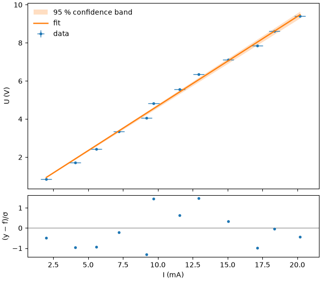
A resistor is characterized with a voltmeter and an ammeter. Both readings have uncertainties, the current even more than the voltage. An ordinary fit treats x as exact and underestimates the uncertainty of the resistance. With xerr, fitwise uses orthogonal distance regression, which accounts for the errors in both variables.

import numpy as np

import fitwise as fw

rng = np.random.default_rng(12)
current_true = np.linspace(2, 20, 12)  # mA
R_true = 0.47  # kΩ, so U = R·I comes out in V
u_I, u_U = 0.4, 0.05  # instrument uncertainties: mA and V
current = current_true + rng.normal(0, u_I, current_true.size)
voltage = R_true * current_true + rng.normal(0, u_U, current_true.size)

ohm = "R*x"

Ordinary fit, current treated as exact. The χ² warning says that the voltage errors alone cannot explain the scatter:

import warnings

with warnings.catch_warnings(record=True):
    ordinary = fw.fit(ohm, current, voltage, yerr=u_U)
print(ordinary)

Model:      y = R*x
Method:     Linear least squares (direct) (auto: linear in the parameters)
Converged:  yes (2 evals)
Data:       12 points, yerr given (absolute)
Start:      R: not needed (linear model)

Parameter    Value   ± Std.Err    Rel.   Bounds
R           0.4688      0.0012   0.2 %   –

χ²/ndf = 13.4 (11 dof, p = 6.4e-26)    R² = 0.9957    AIC = 32.1
Warnings:   ! χ²/ndf = 13.4 is too large for 11 degrees of freedom (p = 6.4e-26): the model does not describe the data, or yerr is underestimated

With xerr the fit is consistent, and the uncertainty of R is realistic:

odr = fw.fit(ohm, current, voltage, yerr=u_U, xerr=u_I)
print(odr)

Model:      y = R*x
Method:     Orthogonal distance regression (odrpack) (auto: xerr given)
Converged:  yes (31 evals)
Data:       12 points, xerr and yerr given (absolute)
Start:      R: from ordinary fit (linear model)

Parameter    Value   ± Std.Err    Rel.   Bounds
R           0.4692      0.0045   1.0 %   –

χ²/ndf = 0.886 (11 dof, p = 0.55)    R² = 0.9957    AIC = -0.5
Warnings:   none

The plot shows error bars in both directions. The residuals are normalized by the effective uncertainty √(yerr² + (R·xerr)²).

fig, axes = odr.plot()
axes[0].set_ylabel("U (V)")
axes[1].set_xlabel("I (mA)")

Text(0.5, 18.503588541666666, 'I (mA)')

for label, r in [("ordinary", ordinary), ("ODR", odr)]:
    R = r.params["R"]
    print(f"{label:8s} R = {1000 * R.value:.1f} ± {1000 * R.stderr:.1f} Ω   (true: 470 Ω)")

ordinary R = 468.8 ± 1.2 Ω   (true: 470 Ω)
ODR      R = 469.2 ± 4.5 Ω   (true: 470 Ω)