Damped pendulum

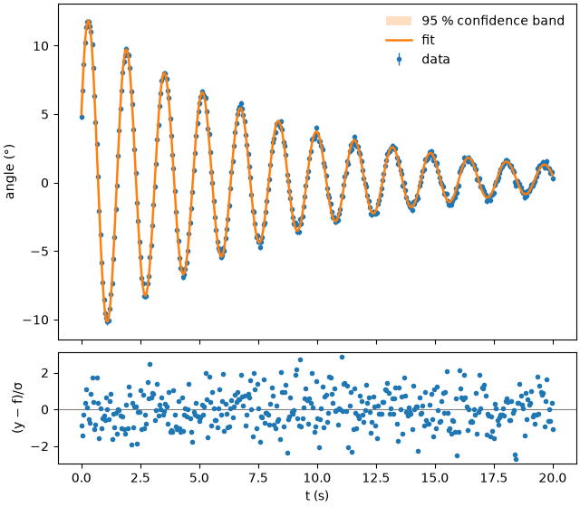
The angle of a pendulum is recorded with a rotary encoder. The oscillation decays exponentially; the encoder has a small zero offset. Frequency, phase and decay time are estimated automatically from a periodogram.

import numpy as np

import fitwise as fw

rng = np.random.default_rng(5)
t = np.linspace(0, 20, 400)  # s
angle = 12 * np.exp(-t / 8) * np.sin(2 * np.pi * 0.62 * t + 0.4) + 0.3 + rng.normal(0, 0.2, t.size)

result = fw.fit(fw.models.damped_sine + fw.models.constant, t, angle, yerr=0.2)
print(result)

Model:      damped_sine(x; amp, freq, phase, tau) + constant(x; c)
Method:     Trust Region Reflective (scipy least_squares) (auto: nonlinear)
Converged:  yes (16 evals)
Data:       400 points, yerr given (absolute)
Start:      amp, freq, phase, tau: periodogram · c: edge baseline

Parameter     Value   ± Std.Err    Rel.   Bounds
amp          12.007       0.045   0.4 %   –
freq        0.61991     0.00012   0.0 %   –
phase        0.4023      0.0039   1.0 %   –
tau           7.986       0.046   0.6 %   –
c             0.290       0.010   3.5 %   –

χ²/ndf = 0.938 (395 dof, p = 0.81)    R² = 0.9975    AIC = -20.6
Correlations > 0.5:  freq–phase (-0.73), amp–tau (-0.72)
Warnings:   none

fig, axes = result.plot()
axes[0].set_ylabel("angle (°)")
axes[1].set_xlabel("t (s)")

Text(0.5, 18.503588541666666, 't (s)')

The quality factor of the pendulum is Q = π f τ. as_ufloat() returns the parameters as correlated values of the uncertainties package, so the error propagation automatically includes the correlation between f and τ:

u = result.params.as_ufloat()
Q = np.pi * u["freq"] * u["tau"]
print(f"Q = {Q:.1uS}")

Q = 15.55(9)

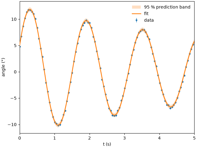
The 95 % prediction band shows where new readings of the encoder are expected:

fig, axes = result.plot(band="prediction", residuals=False)
axes[0].set_xlim(0, 5)
axes[0].set_ylabel("angle (°)")
axes[0].set_xlabel("t (s)")

Text(0.5, 18.503588541666666, 't (s)')