Two peaks on a sloped background

A spectrum with two overlapping emission lines on a linear background. Models are combined with +. Parameter names that occur twice get automatic prefixes; to choose your own names, use with_prefix().

The wavelength is measured relative to the center of the spectrum (655 nm). The intercept of the background is then the background in the spectrum. With absolute wavelengths it would be the background at 0 nm, an extrapolation over 650 nm, and slope and intercept would be almost fully correlated; fitwise would warn about that.

import numpy as np

import fitwise as fw
from fitwise.models import gaussian, linear

rng = np.random.default_rng(10)
wavelength = np.linspace(640, 670, 300)  # nm
intensity = (
    gaussian(wavelength, 820, 651.2, 1.1)
    + gaussian(wavelength, 310, 655.0, 1.4)
    + 2.5 * (wavelength - 640)
    + 40
)
intensity = rng.poisson(intensity).astype(float)
shift = wavelength - 655.0  # nm relative to the center

model = gaussian.with_prefix("a_") + gaussian.with_prefix("b_") + linear
print(model.param_names)

('a_amp', 'a_cen', 'a_sigma', 'b_amp', 'b_cen', 'b_sigma', 'slope', 'intercept')

The starting values come from a sequential estimate: background from the edges, then the strongest peak, then the second peak on what remains.

result = fw.fit(model, shift, intensity, yerr=np.sqrt(intensity))
print(result)

Model:      gaussian(x; a_amp, a_cen, a_sigma) + gaussian(x; b_amp, b_cen, b_sigma) + linear(x; slope, intercept)
Method:     Trust Region Reflective (scipy least_squares) (auto: nonlinear)
Converged:  yes (31 evals)
Data:       300 points, yerr given (absolute)
Start:      a_amp, a_cen, a_sigma, b_amp, b_cen, b_sigma: peak heuristic · slope, intercept: edge baseline

Parameter    Value   ± Std.Err     Rel.   Bounds
a_amp        821.0         7.8    0.9 %   –
a_cen       -3.805       0.015    0.4 %   –
a_sigma      1.081       0.011    1.0 %   –
b_amp        310.4         4.6    1.5 %   –
b_cen       -0.057       0.039   67.4 %   –
b_sigma      1.441       0.033    2.3 %   –
slope        2.513       0.058    2.3 %   –
intercept    76.50        0.62    0.8 %   –

χ²/ndf = 0.916 (292 dof, p = 0.85)    R² = 0.9907    AIC = -18.4
Correlations > 0.5:  a_cen–b_cen (+0.71), b_cen–b_sigma (-0.70), a_cen–b_sigma (-0.66), a_sigma–b_cen (+0.64), a_cen–a_sigma (+0.60), a_sigma–b_sigma (-0.53)
Warnings:   none

fig, axes = result.plot()
x = np.linspace(-15, 15, 600)
p = result.params.values_dict()
background = linear.eval(x, p)
for prefix, color in [("a_", "C2"), ("b_", "C3")]:
    peak = gaussian.with_prefix(prefix).eval(x, p)
    axes[0].fill_between(x, background, background + peak, color=color, alpha=0.3, lw=0)
axes[0].set_ylabel("counts")
axes[1].set_xlabel("wavelength − 655 nm")

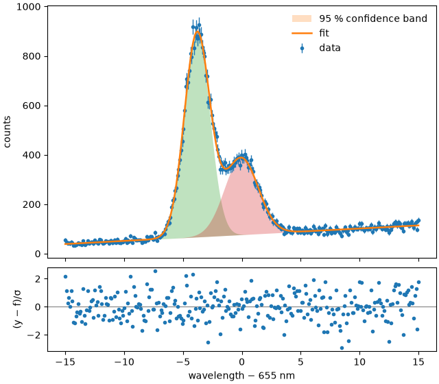
Text(0.5, 18.503588541666666, 'wavelength − 655 nm')

Line positions in absolute wavelength:

for prefix in ("a_", "b_"):
    cen = result.params[prefix + "cen"]
    print(f"line {prefix[0]}: {655 + cen.value:.3f} ± {cen.stderr:.3f} nm")

line a: 651.195 ± 0.015 nm
line b: 654.943 ± 0.039 nm

The line ratio with its uncertainty. as_ufloat() takes the correlation of the two amplitudes into account automatically:

u = result.params.as_ufloat()
ratio = u["b_amp"] / u["a_amp"]
print(f"I_b / I_a = {ratio:.2uS}")

I_b / I_a = 0.3781(62)