Resonance curve

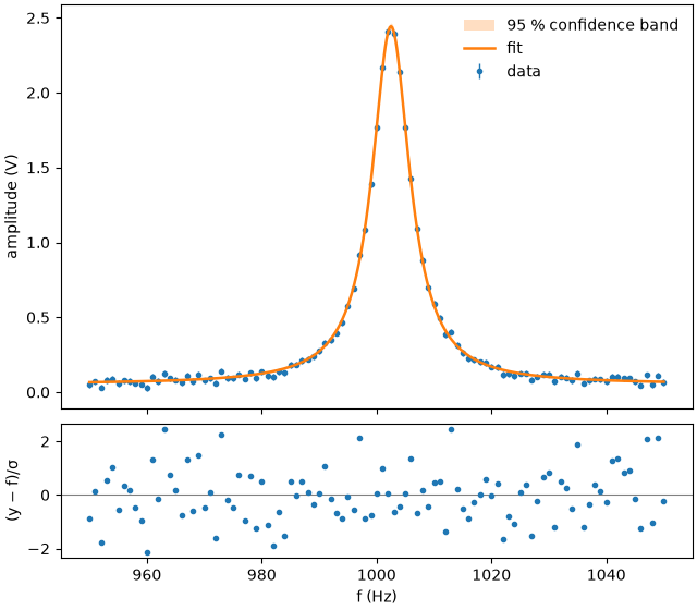
The amplitude of a driven oscillator near resonance is approximately Lorentzian. The quality factor follows from the resonance frequency and the width: Q = f₀ / (2γ), where γ is the half width at half maximum. The detector has a small constant offset.

import numpy as np

import fitwise as fw

rng = np.random.default_rng(9)
f = np.linspace(950, 1050, 101)  # Hz
amplitude = 2.4 * 4.0**2 / ((f - 1002.5) ** 2 + 4.0**2) + 0.05 + rng.normal(0, 0.02, f.size)

result = fw.fit(fw.models.lorentzian + fw.models.constant, f, amplitude, yerr=0.02)
print(result)

Model:      lorentzian(x; amp, cen, gamma) + constant(x; c)
Method:     Trust Region Reflective (scipy least_squares) (auto: nonlinear)
Converged:  yes (24 evals)
Data:       101 points, yerr given (absolute)
Start:      amp, cen, gamma: peak heuristic · c: edge baseline

Parameter      Value   ± Std.Err    Rel.   Bounds
amp            2.392       0.011   0.5 %   –
cen         1002.499       0.019   0.0 %   –
gamma          3.984       0.030   0.8 %   –
c             0.0521      0.0026   4.9 %   –

χ²/ndf = 1.03 (97 dof, p = 0.41)    R² = 0.9986    AIC = 6.4
Correlations > 0.5:  amp–gamma (-0.60)
Warnings:   none

f0, gamma = result.params["cen"], result.params["gamma"]
Q = f0.value / (2 * gamma.value)
print(
    f"f0 = {f0.value:.2f} ± {f0.stderr:.2f} Hz,  Q = {Q:.0f} ± {Q * gamma.stderr / gamma.value:.0f}"
)

f0 = 1002.50 ± 0.02 Hz,  Q = 126 ± 1

fig, axes = result.plot()
axes[0].set_ylabel("amplitude (V)")
axes[1].set_xlabel("f (Hz)")

Text(0.5, 18.503588541666666, 'f (Hz)')