Arrhenius law with your own function

Any Python function can be a model. Here the rate constant of a reaction is measured at several temperatures and described by the Arrhenius law k = A · exp(−Eₐ / RT).

Your own functions have no built-in heuristic for starting values. Default values in the signature are used instead; they only need to be of the right order of magnitude.

import numpy as np

import fitwise as fw

R = 8.314  # J/(mol K)


def arrhenius(T, A=1e10, Ea=50e3):
    """Rate constant in 1/s; T in K, Ea in J/mol."""
    return A * np.exp(-Ea / (R * T))


rng = np.random.default_rng(7)
T = np.linspace(290, 360, 8)
k_true = arrhenius(T, A=4.2e12, Ea=78e3)
k = k_true * (1 + rng.normal(0, 0.03, T.size))  # 3 % relative uncertainty
dk = 0.03 * k

result = fw.fit(arrhenius, T, k, yerr=dk)
print(result)

Model:      arrhenius(x; A, Ea)
Method:     Trust Region Reflective (scipy least_squares) (auto: nonlinear)
Converged:  yes (60 evals)
Data:       8 points, yerr given (absolute)
Start:      A, Ea: signature default

Parameter      Value   ± Std.Err     Rel.   Bounds
A           4.41e+12    0.67e+12   15.2 %   –
Ea             78140         410    0.5 %   –

χ²/ndf = 0.607 (6 dof, p = 0.73)    R² = 0.99944    AIC = -2.3
Correlations > 0.5:  A–Ea (+1.00)
Warnings:   none

The parameters differ by 8 orders of magnitude. fitwise normalizes them internally, so the solver is not affected. A and Eₐ are strongly correlated (see the Correlations line of the report), which is typical for the Arrhenius law: a larger Eₐ can be compensated by a larger A. Use the covariance when you compute something from both.

The classic Arrhenius plot shows k on a log scale over 1/T, where the law is a straight line. result.eval evaluates the fitted model at any temperature:

import matplotlib.pyplot as plt

T_fine = np.linspace(285, 365, 200)
fig, ax = plt.subplots()
ax.errorbar(1000 / T, k, yerr=dk, fmt="o", label="data")
ax.plot(1000 / T_fine, result.eval(T_fine), label="fit")
ax.set_yscale("log")
ax.set_xlabel("1000 / T (1/K)")
ax.set_ylabel("k (1/s)")
ax.legend()

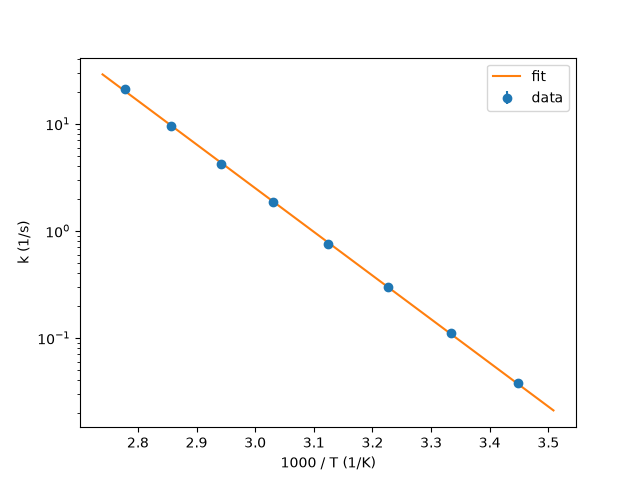
<matplotlib.legend.Legend object at 0x7fb59ef71100>

Ea = result.params["Ea"]
print(f"Ea = {Ea.value / 1e3:.1f} ± {Ea.stderr / 1e3:.1f} kJ/mol")

Ea = 78.1 ± 0.4 kJ/mol