Calibration line

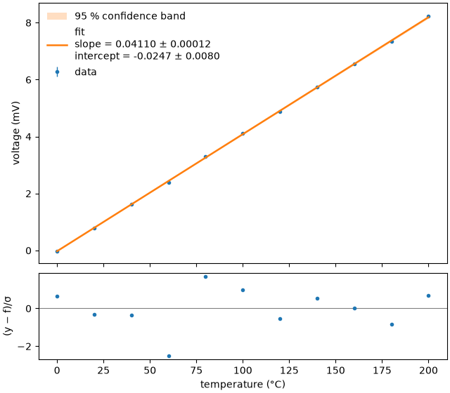
A thermocouple voltage is calibrated against reference temperatures. The model is a straight line; each voltage reading has its own uncertainty.

import numpy as np

import fitwise as fw

rng = np.random.default_rng(2)
temperature = np.array([0.0, 20, 40, 60, 80, 100, 120, 140, 160, 180, 200])  # °C
u_volt = 0.010 + 0.0002 * temperature  # mV, larger at high temperatures
voltage = 0.0410 * temperature - 0.02 + rng.normal(0, u_volt)

result = fw.fit(fw.models.linear, temperature, voltage, yerr=u_volt)
print(result)

Model:      linear(x; slope, intercept)
Method:     Linear least squares (direct) (auto: linear in the parameters)
Converged:  yes (3 evals)
Data:       11 points, yerr given (absolute)
Start:      slope, intercept: not needed (linear model)

Parameter     Value   ± Std.Err     Rel.   Bounds
slope       0.04110     0.00012    0.3 %   –
intercept   -0.0247      0.0080   32.2 %   –

χ²/ndf = 1.38 (9 dof, p = 0.19)    R² = 0.99989    AIC = 5.3
Correlations > 0.5:  slope–intercept (-0.62)
Warnings:   none

The slope is the sensitivity of the thermocouple in mV/°C. Note the strong negative correlation between slope and intercept, listed in the report: both are estimated from the same points, so their errors are not independent.

fig, axes = result.plot(show_params=True)
axes[0].set_ylabel("voltage (mV)")
axes[1].set_xlabel("temperature (°C)")

Text(0.5, 18.503588541666666, 'temperature (°C)')

Because the uncertainties were given, χ²/ndf tests whether they are realistic. A value near 1 means the line describes the data within their errors.

print(f"χ²/ndf = {result.redchi:.2f}, p = {result.pvalue:.2f}")

χ²/ndf = 1.38, p = 0.19