Solitons: the Korteweg-de Vries and Nonlinear Schrödinger Equations
A soliton is a solitary wave that keeps its shape while it travels, and that survives collisions with other solitons. Solitons exist where nonlinearity and dispersion balance each other. The two classic examples are the Korteweg-de Vries (KdV) equation for waves on shallow water,
and the nonlinear Schrödinger (NLS) equation for wave envelopes in optical fibers,
Both have the form \(\partial_t u = L u + N(u)\) with a stiff linear part \(L\) (the highest derivative) and a nonlinear part \(N\) that is not stiff. Explicit time stepping schemes are limited to tiny steps by \(L\). The exponential time differencing schemes of numgrids integrate the linear part exactly and only the nonlinear part with a Runge-Kutta scheme: evolve(..., linear=L, method="ETDRK4", dt=...).
In this notebook we
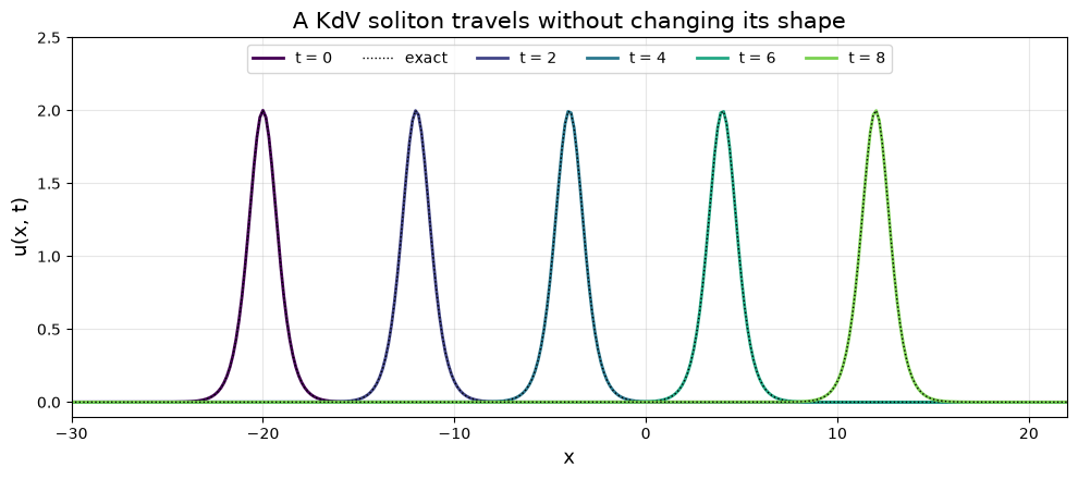
follow a KdV soliton and compare with the exact solution,
let two KdV solitons collide and measure their phase shifts and the conserved quantities,
compare the cost with explicit Runge-Kutta methods,
solve the NLS equation for a bright soliton and for a “breathing” second-order soliton.
Setup
Solitons decay exponentially, so a periodic grid that is large enough serves as the real line. Fourier differentiation is spectrally accurate there. The nonlinear term of the KdV equation is written in the conservative form \(-6\,u\,u_x = -3\,(u^2)_x\).
[1]:
import time

import numpy as np
import matplotlib.pyplot as plt
from numgrids import *

grid = Grid(x=periodic(512, -40, 40))
x = grid.coords
D = grid.diff_operator()

linear = -grid.diff_operator(3)              # the stiff linear part: -u_xxx


def nonlinear(t, u):                         # the nonlinear part: -6 u u_x
    return -3 * D(u**2)

print(grid)
Grid(shape=(512,), ndims=1, axes=[
    EquidistantAxis(num_points=512, low=-40, high=40, periodic=True, name='x')
])
A Single Soliton
The KdV equation has the solutions
for any speed \(c > 0\): taller solitons are narrower and faster. We start one with \(c = 4\) and compare with the exact solution. The conserved quantities mass \(\int u\,dx\) and momentum \(\int u^2 dx\) of the soliton are \(2\sqrt{c} = 4\) and \(\tfrac23 c^{3/2} = 5.333\ldots\)
[2]:
def soliton(t, c=4.0, x0=-20.0):
    return c / 2 / np.cosh(np.sqrt(c) / 2 * (x - x0 - c * t))**2


times = np.linspace(0, 8, 5)
single = evolve(grid, nonlinear, soliton(0), t_span=(0, 8), t_eval=times,
                linear=linear, method="ETDRK4", dt=0.005)

print(single.message)
print("   t    max. error     mass           momentum")
for t, u in zip(single.t, single.u):
    print(f"{t:4.0f}    {np.abs(u - soliton(t)).max():.2e}    {grid.integrate(u):.10f}   {grid.integrate(u**2):.8f}")
The integration reached the end of the time interval with 1600 steps of ETDRK4.
   t    max. error     mass           momentum
   0    0.00e+00    4.0000000000   5.33333333
   2    1.53e-05    4.0000000000   5.33332307
   4    4.62e-05    4.0000000000   5.33331281
   6    9.18e-05    4.0000000000   5.33330254
   8    1.55e-04    4.0000000000   5.33329228
[3]:
fig, ax = plt.subplots(figsize=(10, 4.5))
cmap = plt.cm.viridis
for i, (t, u) in enumerate(zip(single.t, single.u)):
    ax.plot(x, u, color=cmap(i / len(times)), linewidth=2, label=f"t = {t:.0f}")
    ax.plot(x, soliton(t), color="k", linestyle=":", linewidth=1, label="exact" if i == 0 else None)
ax.set_xlim(-30, 22)
ax.set_ylim(-0.1, 2.5)
ax.set_xlabel("x", fontsize=13)
ax.set_ylabel("u(x, t)", fontsize=13)
ax.set_title("A KdV soliton travels without changing its shape", fontsize=15)
ax.legend(fontsize=10, ncol=6, loc="upper center")
ax.grid(True, alpha=0.3)
fig.tight_layout()
plt.show()
Two Solitons Collide
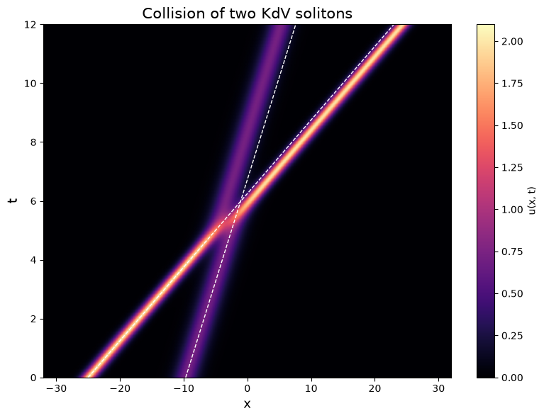
A fast soliton catches up with a slow one. For a nonlinear equation one would expect a complicated interaction, but the two solitons emerge unchanged. The only trace of the collision is a phase shift: the fast soliton has jumped forward, the slow one backward.
The exact two-soliton solution is known (Hirota):
with the speeds \(c_i = k_i^2\). We use it as initial condition and as reference.
[4]:
k1, k2 = 2.0, 1.2                # speeds 4 and 1.44
x1, x2 = -25.0, -12.0


def two_solitons(t):
    e1 = k1 * (x - k1**2 * t - x1)
    e2 = k2 * (x - k2**2 * t - x2)
    terms = np.array([0 * x, e1, e2, e1 + e2 + 2 * np.log((k1 - k2) / (k1 + k2))])
    w = np.exp(terms - terms.max(axis=0))                # scaled, to avoid overflow
    F = w.sum(axis=0)
    F_x = k1 * w[1] + k2 * w[2] + (k1 + k2) * w[3]
    F_xx = k1**2 * w[1] + k2**2 * w[2] + (k1 + k2)**2 * w[3]
    return 2 * (F_xx / F - (F_x / F)**2)


times = np.linspace(0, 12, 241)
start = time.perf_counter()
collision = evolve(grid, nonlinear, two_solitons(0), t_span=(0, 12), t_eval=times,
                   linear=linear, method="ETDRK4", dt=0.005)
print(f"{collision.message}  ({time.perf_counter() - start:.1f} s)")
print(f"largest deviation from the exact solution: {np.abs(collision.final - two_solitons(12)).max():.1e}")
The integration reached the end of the time interval with 2400 steps of ETDRK4.  (2.5 s)
largest deviation from the exact solution: 2.7e-04
Space-time picture
The dashed lines are the paths the solitons would take without the collision.
[5]:
shift = 2 * np.log((k1 + k2) / (k1 - k2))        # the solitons are displaced by shift / k

fig, ax = plt.subplots(figsize=(8, 6))
im = ax.pcolormesh(x, times, collision.u, cmap="magma", shading="gouraud", vmin=0, vmax=2.1)
ax.plot(x1 + k1**2 * times, times, color="white", linestyle="--", linewidth=1)
ax.plot(x2 + shift / k2 + k2**2 * times, times, color="white", linestyle="--", linewidth=1)
ax.set_xlim(-32, 32)
ax.set_xlabel("x", fontsize=13)
ax.set_ylabel("t", fontsize=13)
ax.set_title("Collision of two KdV solitons", fontsize=15)
fig.colorbar(im, ax=ax, label="u(x, t)")
fig.tight_layout()
plt.show()
Phase shifts
The theory predicts that the fast soliton is displaced by \(+\frac{2}{k_1}\ln\frac{k_1 + k_2}{k_1 - k_2}\) and the slow one by \(-\frac{2}{k_2}\ln\frac{k_1 + k_2}{k_1 - k_2}\). We locate the two maxima of the final state by spectral interpolation and compare with the positions of undisturbed solitons.
[6]:
fine = np.linspace(-40, 40, 80001)
u_end = grid.interpolate(collision.final, fine)

peak_fast = fine[np.argmax(u_end)]
behind = fine < peak_fast - 5
peak_slow = fine[behind][np.argmax(u_end[behind])]

t_end = times[-1]
print("            measured    theory")
print(f"fast:      {peak_fast - (x1 + k1**2 * t_end):9.4f} {shift / k1:9.4f}")
print(f"slow:      {peak_slow - (x2 + shift / k2 + k2**2 * t_end):9.4f} {-shift / k2:9.4f}")
print(f"heights:   {u_end.max():.5f}, {u_end[behind].max():.5f}    (before: {k1**2 / 2:.5f}, {k2**2 / 2:.5f})")
            measured    theory
fast:         1.3860    1.3863
slow:        -2.3105   -2.3105
heights:   1.99998, 0.72000    (before: 2.00000, 0.72000)
Conserved quantities
The KdV equation has infinitely many conserved quantities. The first three are mass, momentum and energy,
grid.integrate evaluates them with spectral accuracy. They stay constant throughout the collision:
[7]:
print("    t     mass            momentum      energy")
for i in range(0, len(times), 60):
    u = collision.u[i]
    print(f"{times[i]:5.1f}    {grid.integrate(u):.10f}    {grid.integrate(u**2):.7f}"
          f"     {grid.integrate(u**3 - 0.5 * D(u)**2):.7f}")
    t     mass            momentum      energy
  0.0    6.4000000000    6.4853333     6.8976640
  3.0    6.4000000000    6.4853180     6.8976332
  6.0    6.4000000000    6.4853105     6.8976178
  9.0    6.4000000000    6.4852960     6.8975895
 12.0    6.4000000000    6.4852806     6.8975587
Step Sizes and Cost
How large can the time step be? The third derivative has eigenvalues up to \(k_\text{max}^3\) on the imaginary axis, where \(k_\text{max} = \pi / \Delta x\) is the largest wave number of the grid. An explicit Runge-Kutta method is only stable if the step is of the order \(1/k_\text{max}^3\), however smooth the solution is. The exponential schemes have no such limit: their step is chosen for the accuracy of the nonlinear part.
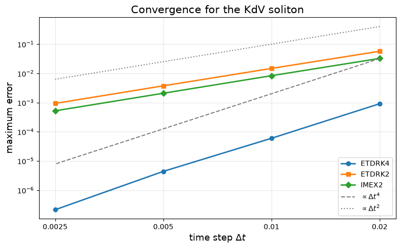
We integrate a soliton over a short time with the explicit methods of scipy.integrate.solve_ivp (with the complete right-hand side) and with three schemes for the split problem: ETDRK4 (order 4), ETDRK2 (order 2), and the implicit-explicit scheme IMEX2 (order 2), which treats the linear part implicitly.
[8]:
small = Grid(x=periodic(256, -20, 20))
xs = small.coords
Ds, D3s = small.diff_operator(), small.diff_operator(3)
profile = lambda t: 2 / np.cosh(xs + 8 - 4 * t)**2            # the soliton with c = 4
T = 0.5

k_max = np.pi / (xs[1] - xs[0])
print(f"largest eigenvalue of the linear part: {k_max**3:.0f}\n")
print("method              steps   evaluations    time     error")

for method, options in [("RK45", dict(rtol=1e-6, atol=1e-9)), ("DOP853", dict(rtol=1e-8, atol=1e-10))]:
    start = time.perf_counter()
    res = evolve(small, lambda t, u: -D3s(u) - 3 * Ds(u**2), profile(0), (0, T), method=method, **options)
    elapsed = time.perf_counter() - start
    print(f"{method:16s} {len(res.sol.t) - 1:8d} {res.sol.nfev:10d}   {elapsed:6.2f} s   "
          f"{np.abs(res.final - profile(T)).max():.1e}")

evaluations = {"ETDRK4": 4, "ETDRK2": 2, "IMEX2": 2}
for method, dt in [("ETDRK4", 0.01), ("ETDRK4", 0.005), ("ETDRK2", 0.001), ("IMEX2", 0.001)]:
    start = time.perf_counter()
    res = evolve(small, lambda t, u: -3 * Ds(u**2), profile(0), (0, T), linear=-D3s, method=method, dt=dt)
    elapsed = time.perf_counter() - start
    steps = round(T / dt)
    print(f"{method + f', dt={dt}':16s} {steps:8d} {evaluations[method] * steps:10d}   {elapsed:6.2f} s   "
          f"{np.abs(res.final - profile(T)).max():.1e}")
largest eigenvalue of the linear part: 8128

method              steps   evaluations    time     error
RK45                 3151      18932     2.24 s   7.1e-07
DOP853                669       8078     0.95 s   8.0e-11
ETDRK4, dt=0.01        50        200     0.02 s   6.0e-05
ETDRK4, dt=0.005      100        400     0.04 s   4.4e-06
ETDRK2, dt=0.001      500       1000     0.10 s   1.5e-04
IMEX2, dt=0.001       500       1000     0.10 s   8.3e-05
The explicit methods need hundreds to thousands of steps for this short time. Their step size is dictated by stability, not by accuracy: looser tolerances would not make them cheaper. ETDRK4 takes a hundred steps for an error of a few \(10^{-6}\), with 20 to 50 times fewer evaluations of the right-hand side.
The errors of the fixed-step schemes decrease with their order when the step is reduced:
[9]:
dts = np.array([0.02, 0.01, 0.005, 0.0025])
errors = {}
for method in ("ETDRK4", "ETDRK2", "IMEX2"):
    errors[method] = [np.abs(evolve(small, lambda t, u: -3 * Ds(u**2), profile(0), (0, T), linear=-D3s,
                                    method=method, dt=dt).final - profile(T)).max() for dt in dts]

fig, ax = plt.subplots(figsize=(8, 5))
for method, marker in zip(errors, "osD"):
    ax.loglog(dts, errors[method], marker=marker, linewidth=2, label=method)
ax.loglog(dts, 2e5 * dts**4, color="gray", linestyle="--", label=r"$\propto \Delta t^4$")
ax.loglog(dts, 1e3 * dts**2, color="gray", linestyle=":", label=r"$\propto \Delta t^2$")
ax.set_xticks(dts)
ax.set_xticklabels([f"{dt:g}" for dt in dts])
ax.minorticks_off()
ax.set_xlabel(r"time step $\Delta t$", fontsize=13)
ax.set_ylabel("maximum error", fontsize=13)
ax.set_title("Convergence for the KdV soliton", fontsize=15)
ax.legend(fontsize=10)
ax.grid(True, alpha=0.3)
fig.tight_layout()
plt.show()

for method in errors:
    orders = np.log2(np.array(errors[method][:-1]) / np.array(errors[method][1:]))
    print(f"{method}: observed orders {np.round(orders, 2)}")
ETDRK4: observed orders [3.93 3.77 4.37]
ETDRK2: observed orders [1.95 1.98 2.  ]
IMEX2: observed orders [1.97 2.   2.  ]
The Nonlinear Schrödinger Equation
The NLS equation has a complex field. Its linear part \(\tfrac{i}{2}\,\partial_x^2\) is the free Schrödinger operator, the nonlinear part is \(i\,|\psi|^2 \psi\). The bright soliton
does not move at all: dispersion and self-focusing cancel exactly, and only the phase rotates. The norm \(\int |\psi|^2 dx = 2\) is conserved. These solitons are narrower than the KdV solitons above, so we take a finer grid.
[10]:
grid = Grid(x=periodic(512, -20, 20))
x = grid.coords
nls_linear = 0.5j * grid.diff_operator(2)


def nls_nonlinear(t, psi):
    return 1j * np.abs(psi)**2 * psi


bright = evolve(grid, nls_nonlinear, 1 / np.cosh(x), t_span=(0, 20), t_eval=np.linspace(0, 20, 5),
                linear=nls_linear, method="ETDRK4", dt=0.02)

print("   t    max. error    norm^2")
for t, psi in zip(bright.t, bright.u):
    print(f"{t:4.0f}    {np.abs(psi - np.exp(0.5j * t) / np.cosh(x)).max():.1e}     {grid.norm(psi)**2:.10f}")
   t    max. error    norm^2
   0    0.0e+00     2.0000000000
   5    3.3e-08     1.9999999998
  10    6.8e-08     1.9999999997
  15    1.0e-07     1.9999999995
  20    1.4e-07     1.9999999993
A breathing soliton
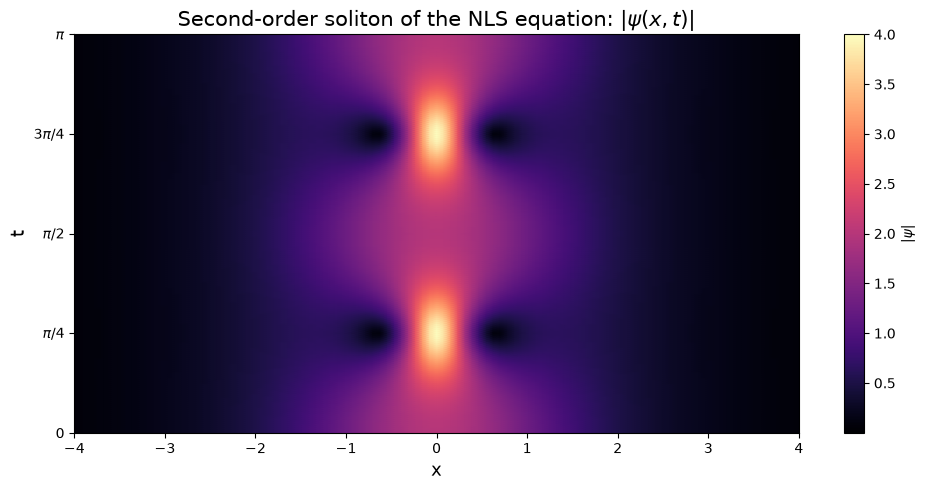
Twice the amplitude, \(\psi(x, 0) = 2 \operatorname{sech}(x)\), gives a bound state of two solitons. It contracts and widens periodically, with the period \(\pi/2\). Satsuma and Yajima found the exact solution
whose maximum reaches \(|\psi| = 4\) at \(t = \pi/4\).
[11]:
def breather(t):
    return (4 * np.exp(0.5j * t) * (np.cosh(3 * x) + 3 * np.exp(4j * t) * np.cosh(x))
            / (np.cosh(4 * x) + 4 * np.cosh(2 * x) + 3 * np.cos(4 * t)))


times = np.linspace(0, np.pi, 201)
breathing = evolve(grid, nls_nonlinear, 2 / np.cosh(x), t_span=(0, np.pi), t_eval=times,
                   linear=nls_linear, method="ETDRK4", dt=0.002)

print("   t      max. error    max |psi|    norm^2")
for i in (0, 50, 100, 200):
    psi = breathing.u[i]
    print(f"{times[i]:6.4f}    {np.abs(psi - breather(times[i])).max():.1e}     {np.abs(psi).max():.6f}"
          f"    {grid.norm(psi)**2:.9f}")
   t      max. error    max |psi|    norm^2
0.0000    2.2e-16     2.000000    8.000000000
0.7854    6.3e-07     4.000001    8.000000020
1.5708    1.8e-07     2.000000    7.999999994
3.1416    4.2e-07     2.000000    7.999999989
[12]:
fig, ax = plt.subplots(figsize=(10, 5))
im = ax.pcolormesh(x, times, np.abs(breathing.u), cmap="magma", shading="gouraud")
ax.set_xlim(-4, 4)
ax.set_yticks([0, np.pi / 4, np.pi / 2, 3 * np.pi / 4, np.pi])
ax.set_yticklabels(["0", r"$\pi/4$", r"$\pi/2$", r"$3\pi/4$", r"$\pi$"])
ax.set_xlabel("x", fontsize=13)
ax.set_ylabel("t", fontsize=13)
ax.set_title(r"Second-order soliton of the NLS equation: $|\psi(x, t)|$", fontsize=15)
fig.colorbar(im, ax=ax, label=r"$|\psi|$")
fig.tight_layout()
plt.show()
Summary
evolve(grid, N, u0, t_span, linear=L, method="ETDRK4", dt=...)integrates stiff semilinear problems \(\partial_t u = L u + N(t, u)\): the linear part exactly, the nonlinear part with a Runge-Kutta scheme of order 4.The time step is limited by accuracy, not by the stiffness of the linear part. For the KdV soliton this saves a factor of 20 to 50 in evaluations compared to explicit methods.
On periodic grids, linear parts with constant coefficients are handled in Fourier space, with fast Fourier transforms.
Complex fields work the same way: the NLS solitons are reproduced to 6 or more digits, with conserved norm.
ETDRK2andIMEX2are second-order alternatives;IMEX2only solves linear systems and is meant for large problems on grids with boundaries.