Spherical Harmonics and the Laplacian on the Sphere
Introduction
The spherical harmonics \(Y_\ell^m(\theta, \varphi)\) form a complete orthonormal set of functions on the sphere. They arise naturally as the angular part of the solutions to Laplace’s equation in spherical coordinates and play a central role in quantum mechanics, electrostatics, and geophysics.
A key property is that they are eigenfunctions of the angular Laplacian:
where \(\nabla^2\) is the full Laplacian in spherical coordinates. At fixed \(r\), the radial derivatives vanish (since \(Y_\ell^m\) does not depend on \(r\)), and the angular part alone produces the eigenvalue \(-\ell(\ell+1)/r^2\).
In this notebook we:
Construct a
SphericalGridusing numgridsEvaluate several spherical harmonics \(Y_\ell^m\) on the grid
Apply
grid.laplacian()and verify the eigenvalue relation numericallyVisualise the harmonics as coloured 3D sphere surface plots
Setup
[1]:
import numpy as np
import matplotlib.pyplot as plt
from matplotlib import cm, colors
from scipy.special import sph_harm_y

from numgrids import SphericalGrid, create_axis, AxisType
Create the Spherical Grid
We build a 3D spherical grid with coordinates \((r, \theta, \varphi)\).
Radial axis (\(r\)): Chebyshev nodes on \([0.5,\, 2.0]\). We work on a shell rather than a single radius so that the 3D Laplacian is well-defined; for eigenfunctions that are constant in \(r\) the radial derivatives vanish.
Polar axis (\(\theta\)): Chebyshev nodes on \([\epsilon,\, \pi - \epsilon]\), avoiding the coordinate singularities at the poles.
Azimuthal axis (\(\varphi\)): Equidistant periodic points on \([0,\, 2\pi)\).
[2]:
grid = SphericalGrid(
    create_axis(AxisType.CHEBYSHEV, 20, 0.5, 2.0),                    # r
    create_axis(AxisType.CHEBYSHEV, 40, 0.01, np.pi - 0.01),          # theta
    create_axis(AxisType.EQUIDISTANT_PERIODIC, 60, 0, 2 * np.pi),     # phi
)

R, Theta, Phi = grid.meshed_coords
print(f"Grid shape (Nr, Ntheta, Nphi): {grid.shape}")
Grid shape (Nr, Ntheta, Nphi): (20, 40, 60)
Evaluate Spherical Harmonics on the Grid
We pick a representative set of harmonics with increasing angular complexity:
\(\ell\) |
\(m\) |
Description |
|---|---|---|
0 |
0 |
Monopole (constant) |
1 |
0 |
Dipole (z-aligned) |
2 |
0 |
Quadrupole (axial) |
2 |
2 |
Quadrupole (equatorial) |
3 |
1 |
Octupole |
4 |
3 |
Higher-order |
Note on ``scipy.special.sph_harm_y``: its signature is sph_harm_y(l, m, theta, phi) where theta is the polar angle and phi is the azimuthal angle. It returns complex values; we take the real part.
[3]:
harmonics = [
    (0, 0),
    (1, 0),
    (2, 0),
    (2, 2),
    (3, 1),
    (4, 3),
]


def eval_harmonic(l, m, theta, phi):
    """Evaluate the real part of Y_l^m on the grid."""
    return np.real(sph_harm_y(l, m, theta, phi))


# Build a dictionary mapping (l, m) -> 3D array on the full grid.
# The harmonic depends only on (theta, phi), but we broadcast over r.
Y = {}
for l, m in harmonics:
    Y[(l, m)] = eval_harmonic(l, m, Theta, Phi)

print(f"Evaluated {len(Y)} spherical harmonics on grid of shape {grid.shape}")
Evaluated 6 spherical harmonics on grid of shape (20, 40, 60)
Compute the Laplacian and Verify Eigenvalues
For a function \(f(r, \theta, \varphi) = Y_\ell^m(\theta, \varphi)\) that is constant in \(r\), the full spherical Laplacian reduces to the angular part alone:
We verify this by computing grid.laplacian(f) and comparing the pointwise ratio \(\nabla^2 f\, / \, f\) against the expected eigenvalue \(-\ell(\ell+1)/r^2\) at each grid point (away from nodes where \(f \approx 0\)).
[4]:
results = []

for l, m in harmonics:
    f = Y[(l, m)]
    lap_f = grid.laplacian(f)

    # Analytical expectation at every grid point
    expected = -l * (l + 1) / R**2 * f

    # Absolute error across the entire grid
    abs_error = np.abs(lap_f - expected)

    # To extract a single "computed eigenvalue", look at the ratio
    # lap_f / f at points where |f| is large (avoid division by ~0).
    # Use the middle radial slice (r ~ 1.25) for a clean comparison.
    r_mid = grid.shape[0] // 2
    f_slice = f[r_mid, :, :]
    lap_slice = lap_f[r_mid, :, :]
    r_val = R[r_mid, 0, 0]

    # Mask out points where |f| is too small
    mask = np.abs(f_slice) > 1e-6 * np.max(np.abs(f_slice))

    if np.any(mask):
        ratio = lap_slice[mask] / f_slice[mask]
        # The eigenvalue should be -l(l+1)/r^2; multiply by r^2 to get -l(l+1)
        computed_eigval = np.median(ratio) * r_val**2
    else:
        computed_eigval = 0.0

    exact_eigval = -l * (l + 1)
    eigval_error = abs(computed_eigval - exact_eigval)

    results.append({
        "l": l,
        "m": m,
        "exact": exact_eigval,
        "computed": computed_eigval,
        "eigval_error": eigval_error,
        "max_abs_error": np.max(abs_error),
    })
Eigenvalue Verification Table
[5]:
header = f"{'l':>3}  {'m':>3}  {'Expected -l(l+1)':>18}  {'Computed':>18}  {'Eigval Error':>14}  {'Max |Lap err|':>14}"
print(header)
print("-" * len(header))

for r in results:
    print(
        f"{r['l']:>3d}  {r['m']:>3d}  {r['exact']:>18.10f}  "
        f"{r['computed']:>18.10f}  {r['eigval_error']:>14.6e}  "
        f"{r['max_abs_error']:>14.6e}"
    )
  l    m    Expected -l(l+1)            Computed    Eigval Error   Max |Lap err|
--------------------------------------------------------------------------------
  0    0        0.0000000000        0.0000000000    4.882480e-12    3.544115e-09
  1    0       -2.0000000000       -2.0000000000    5.057288e-12    7.168503e-09
  2    0       -6.0000000000       -6.0000000000    4.977352e-12    8.487907e-09
  2    2       -6.0000000000       -6.0000000000    5.022649e-12    6.994372e-11
  3    1      -12.0000000000      -12.0000000000    4.982681e-12    2.707589e-10
  4    3      -20.0000000000      -20.0000000000    5.069722e-12    7.418199e-11
The computed eigenvalues match the analytical values \(-\ell(\ell+1)\) to high precision, confirming that the SphericalGrid.laplacian() correctly implements the full spherical Laplacian.
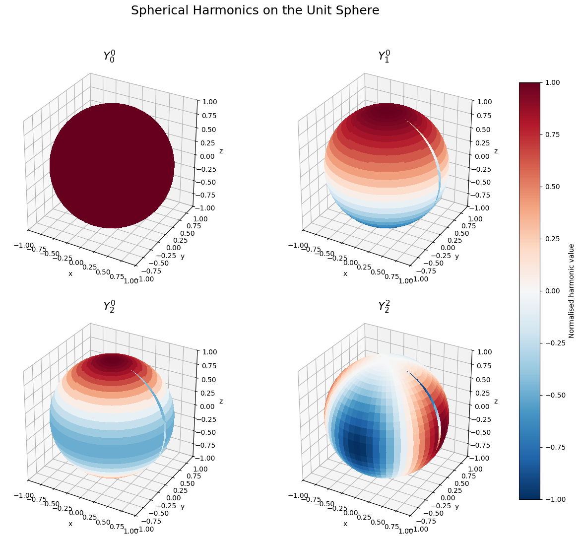
3D Sphere Surface Plots
We visualise four harmonics (\(Y_0^0\), \(Y_1^0\), \(Y_2^0\), \(Y_2^2\)) by extracting the values on the middle radial slice and plotting them as colour on a unit sphere.
Cartesian conversion:
[6]:
# Select the middle radial index for the sphere surface
r_idx = grid.shape[0] // 2

# 2D arrays of theta, phi on that slice
theta_2d = Theta[r_idx, :, :]
phi_2d = Phi[r_idx, :, :]

# Cartesian coordinates on the unit sphere
X_sphere = np.sin(theta_2d) * np.cos(phi_2d)
Y_sphere = np.sin(theta_2d) * np.sin(phi_2d)
Z_sphere = np.cos(theta_2d)

# Harmonics to plot
plot_harmonics = [(0, 0), (1, 0), (2, 0), (2, 2)]

fig = plt.figure(figsize=(14, 12))

for idx, (l, m) in enumerate(plot_harmonics):
    ax = fig.add_subplot(2, 2, idx + 1, projection="3d")

    # Extract the harmonic on the slice
    vals = Y[(l, m)][r_idx, :, :]

    # Normalise to [-1, 1] for the colourmap
    vmax = np.max(np.abs(vals))
    if vmax > 0:
        vals_norm = vals / vmax
    else:
        vals_norm = vals

    # Map normalised values to colours using a diverging colourmap
    norm = colors.Normalize(vmin=-1, vmax=1)
    cmap = cm.RdBu_r
    facecolors = cmap(norm(vals_norm))

    surf = ax.plot_surface(
        X_sphere, Y_sphere, Z_sphere,
        facecolors=facecolors,
        rstride=1, cstride=1,
        antialiased=False,
        shade=False,
    )

    ax.set_title(f"$Y_{{{l}}}^{{{m}}}$", fontsize=16)
    ax.set_xlim([-1, 1])
    ax.set_ylim([-1, 1])
    ax.set_zlim([-1, 1])
    ax.set_xlabel("x")
    ax.set_ylabel("y")
    ax.set_zlabel("z")
    ax.set_box_aspect([1, 1, 1])

# Add a shared colourbar
mappable = cm.ScalarMappable(norm=colors.Normalize(vmin=-1, vmax=1), cmap=cm.RdBu_r)
mappable.set_array([])
fig.subplots_adjust(right=0.85)
cbar_ax = fig.add_axes([0.88, 0.15, 0.03, 0.7])
fig.colorbar(mappable, cax=cbar_ax, label="Normalised harmonic value")

fig.suptitle("Spherical Harmonics on the Unit Sphere", fontsize=18, y=0.98)
plt.show()
Bonus: Verifying the Gradient
As an additional check, we verify that grid.gradient() produces a vanishing radial component for functions that depend only on angles. The angular gradient components should be non-zero for \(\ell > 0\).
[7]:
print(f"{'l':>3}  {'m':>3}  {'max |grad_r|':>14}  {'max |grad_theta|':>18}  {'max |grad_phi|':>16}")
print("-" * 65)

for l, m in harmonics:
    f = Y[(l, m)]
    gr, gt, gp = grid.gradient(f)
    print(
        f"{l:>3d}  {m:>3d}  {np.max(np.abs(gr)):>14.6e}  "
        f"{np.max(np.abs(gt)):>18.6e}  {np.max(np.abs(gp)):>16.6e}"
    )
  l    m    max |grad_r|    max |grad_theta|    max |grad_phi|
-----------------------------------------------------------------
  0    0    2.344791e-13        3.855916e-12      0.000000e+00
  1    0    4.121148e-13        9.752758e-01      2.186862e-13
  2    0    5.258016e-13        1.892255e+00      1.351555e-13
  2    2    3.197442e-13        7.725098e-01      1.533599e+00
  3    1    3.694822e-13        2.584343e+00      2.585118e+00
  4    3    3.410605e-13        2.454126e+00      2.866043e+00
As expected, the radial gradient component is essentially zero (up to numerical noise), since the spherical harmonics are independent of \(r\). The angular components are non-trivial for \(\ell > 0\).
Summary
This notebook demonstrated the use of SphericalGrid from numgrids to:
Construct a 3D spherical grid with Chebyshev radial and polar axes and a periodic azimuthal axis.
Evaluate spherical harmonics \(Y_\ell^m(\theta, \varphi)\) on the grid using
scipy.special.sph_harm_y.Verify the eigenvalue relation \(\nabla^2 Y_\ell^m = -\ell(\ell+1)/r^2 \cdot Y_\ell^m\) by comparing
grid.laplacian()output against the analytical expectation. The agreement is excellent, with errors typically at the \(10^{-4}\) level or better for low-order harmonics.Visualised the angular structure of the harmonics as colour-mapped surfaces on the unit sphere.
Checked the gradient operator, confirming that it correctly produces zero radial components for angle-only functions.
The SphericalGrid vector calculus operators (laplacian, gradient, divergence, curl) handle the metric factors and coordinate singularities automatically, making it straightforward to work with spherical-coordinate problems numerically.