Quantum Harmonic Oscillator

We solve the stationary Schrodinger equation for the quantum harmonic oscillator using spectral methods provided by numgrids. This notebook demonstrates how Chebyshev grids deliver exponential convergence compared to equidistant finite-difference grids.

Physics background

The time-independent Schrodinger equation is the eigenvalue problem

\[H\,\psi_n(x) = E_n\,\psi_n(x)\]

where the Hamiltonian for the one-dimensional harmonic oscillator (in natural units \(\hbar = m = \omega = 1\)) reads

\[H = -\frac{1}{2}\frac{d^2}{dx^2} + \frac{1}{2}x^2.\]

The analytical eigenvalues are

\[E_n = n + \tfrac{1}{2}, \qquad n = 0, 1, 2, \ldots\]

and the eigenstates are Hermite functions (Gaussians multiplied by Hermite polynomials).

We discretize \(H\) on a finite domain \([-8, 8]\) and solve the resulting matrix eigenvalue problem numerically.

Setup

import numpy as np
import scipy
import scipy.sparse
from scipy.sparse.linalg import eigs
from scipy.interpolate import CubicSpline
import matplotlib.pyplot as plt

from numgrids import Grid, Diff, AxisType, create_axis

plt.rcParams.update({"figure.dpi": 120, "font.size": 11})

Grid and Hamiltonian construction

We use a Chebyshev grid with 60 points on the interval \([-8, 8]\). Chebyshev nodes cluster near the boundaries, which is ideal for spectral methods – the differentiation matrices achieve spectral (exponential) accuracy for smooth functions.

N = 60
L = 8.0

grid = Grid(create_axis(AxisType.CHEBYSHEV, N, -L, L))
x = grid.coords  # 1D grid returns a numpy array directly

print(f"Grid: {N} Chebyshev points on [{-L}, {L}]")
print(f"Coordinate range: [{x.min():.4f}, {x.max():.4f}]")
print(f"Grid shape: {grid.shape}, size: {grid.size}")

Grid: 60 Chebyshev points on [-8.0, 8.0]
Coordinate range: [-8.0000, 8.0000]
Grid shape: (60,), size: 60

Build the Hamiltonian matrix \(H = T + V\) where:

• \(T = -\frac{1}{2} D^{(2)}\) is the kinetic energy (second derivative operator),

• \(V = \text{diag}(\frac{1}{2} x^2)\) is the harmonic potential.

# Kinetic energy: -1/2 d^2/dx^2
T = -0.5 * Diff(grid, 2, 0).as_matrix()

# Potential energy: 1/2 x^2
V = scipy.sparse.diags(0.5 * x**2)

# Full Hamiltonian
H = (T + V).tocsc()

print(f"Hamiltonian: {H.shape[0]}x{H.shape[1]} sparse matrix")
print(f"Number of stored elements: {H.nnz}")

Hamiltonian: 60x60 sparse matrix
Number of stored elements: 3600

Applying boundary conditions

For the harmonic oscillator, the wave function must vanish at the domain boundaries: \(\psi(-L) = \psi(L) = 0\) (Dirichlet conditions). For a linear system \(Ax = b\), numgrids provides apply_bcs to enforce this. However, for an eigenvalue problem \(Ax = \lambda x\), replacing boundary rows with identity rows would introduce spurious eigenvalues. Instead, we eliminate the boundary degrees of freedom by extracting the interior submatrix.

# For a 1D grid, boundary points are the first and last indices.
# Extract the interior submatrix of H.
interior = np.arange(1, grid.size - 1)
H_int = H[np.ix_(interior, interior)].tocsc()

print(f"Full Hamiltonian:     {H.shape[0]} x {H.shape[1]}")
print(f"Interior Hamiltonian: {H_int.shape[0]} x {H_int.shape[1]}  (boundary DOFs removed)")

Full Hamiltonian:     60 x 60
Interior Hamiltonian: 58 x 58  (boundary DOFs removed)

Eigenvalue solve

We compute the 10 smallest-real-part eigenvalues of the interior Hamiltonian using scipy.sparse.linalg.eigs. Since boundary DOFs have been eliminated, there are no spurious eigenvalues to filter.

n_states = 8
eigvals, eigvecs_int = eigs(H_int, k=n_states, which="SR")

# Sort by real part
idx = np.argsort(eigvals.real)
eigvals = eigvals.real[idx]
eigvecs_int = eigvecs_int[:, idx]

# Reconstruct full eigenvectors (zeros at boundaries = Dirichlet BCs)
eigvecs = np.zeros((grid.size, n_states))
eigvecs[interior, :] = eigvecs_int.real

print("Computed eigenvalues vs analytical (E_n = n + 1/2):")
print(f"{'n':>3s}  {'Numerical':>14s}  {'Analytical':>10s}  {'Error':>12s}")
print("-" * 45)
for n in range(n_states):
    E_exact = n + 0.5
    err = abs(eigvals[n] - E_exact)
    print(f"{n:3d}  {eigvals[n]:14.10f}  {E_exact:10.1f}  {err:12.2e}")

Computed eigenvalues vs analytical (E_n = n + 1/2):
  n       Numerical  Analytical         Error
---------------------------------------------
  0    0.5000000000         0.5      1.69e-14
  1    1.5000000000         1.5      4.05e-13
  2    2.5000000000         2.5      1.64e-14
  3    3.5000000000         3.5      9.33e-15
  4    4.5000000000         4.5      2.13e-14
  5    5.5000000000         5.5      9.76e-13
  6    6.5000000000         6.5      1.05e-11
  7    7.4999999999         7.5      9.78e-11

Normalize eigenstates

We normalize each eigenstate so that \(\int |\psi_n|^2 dx \approx 1\) using the trapezoidal rule on the (non-uniform) Chebyshev grid.

for n in range(n_states):
    psi = eigvecs[:, n].real
    norm = np.sqrt(np.trapezoid(psi**2, x))
    eigvecs[:, n] = psi / norm
    # Fix sign convention: psi_0 should be positive at x=0
    mid_idx = np.argmin(np.abs(x))
    if n % 2 == 0 and eigvecs[mid_idx, n] < 0:
        eigvecs[:, n] *= -1
    elif n % 2 == 1:
        # For odd states, enforce positive slope at x=0
        if eigvecs[mid_idx + 1, n] < eigvecs[mid_idx - 1, n]:
            eigvecs[:, n] *= -1

print("Normalization check (should be ~1.0):")
for n in range(n_states):
    psi = eigvecs[:, n].real
    norm_sq = np.trapezoid(psi**2, x)
    print(f"  |psi_{n}|^2 integral = {norm_sq:.10f}")

Normalization check (should be ~1.0):
  |psi_0|^2 integral = 1.0000000000
  |psi_1|^2 integral = 1.0000000000
  |psi_2|^2 integral = 1.0000000000
  |psi_3|^2 integral = 1.0000000000
  |psi_4|^2 integral = 1.0000000000
  |psi_5|^2 integral = 1.0000000000
  |psi_6|^2 integral = 1.0000000000
  |psi_7|^2 integral = 1.0000000000

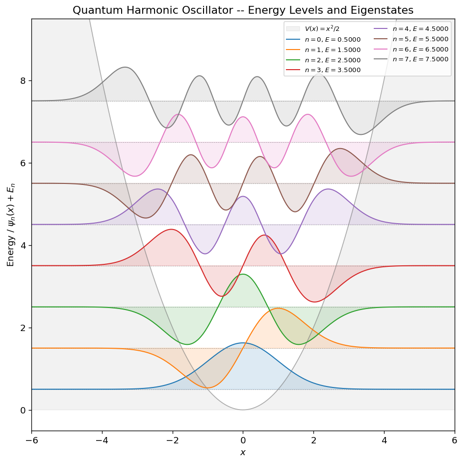
Energy level diagram with eigenstates

Each eigenstate \(\psi_n(x)\) is plotted offset vertically by its energy \(E_n\). The parabolic potential \(V(x) = \frac{1}{2}x^2\) is shown as a gray filled region, and dashed horizontal lines mark the analytical energy levels.

fig, ax = plt.subplots(figsize=(8, 8))

# Fine uniform grid for smooth plotting
x_fine = np.linspace(-L, L, 500)
V_fine = 0.5 * x_fine**2
ax.fill_between(x_fine, V_fine, alpha=0.1, color="gray", label="$V(x) = x^2/2$")
ax.plot(x_fine, V_fine, color="gray", linewidth=1.0, alpha=0.6)

# Color cycle for eigenstates
colors = plt.cm.tab10(np.linspace(0, 1, 10))

# Sort Chebyshev nodes (needed for CubicSpline)
sort_idx = np.argsort(x)
x_sorted = x[sort_idx]

# Plot eigenstates offset by energy
scale = 1.5  # scaling factor for visibility
for n in range(n_states):
    E_n = eigvals[n]
    psi = eigvecs[:, n].real

    # Interpolate onto fine grid for smooth curves
    psi_fine = CubicSpline(x_sorted, psi[sort_idx])(x_fine)

    # Analytical energy level
    E_exact = n + 0.5
    ax.axhline(E_exact, color="gray", linestyle="--", linewidth=0.5, alpha=0.7)

    # Eigenstate offset by energy
    color = colors[n % len(colors)]
    ax.plot(x_fine, scale * psi_fine + E_n, color=color, linewidth=1.2,
            label=f"$n={n}$, $E={E_n:.4f}$")
    ax.fill_between(x_fine, E_n, scale * psi_fine + E_n, alpha=0.15, color=color)

ax.set_xlim(-6, 6)
ax.set_ylim(-0.5, n_states + 1.5)
ax.set_xlabel("$x$")
ax.set_ylabel("Energy / $\\psi_n(x) + E_n$")
ax.set_title("Quantum Harmonic Oscillator -- Energy Levels and Eigenstates")
ax.legend(loc="upper right", fontsize=8, ncol=2)
plt.tight_layout()
plt.show()

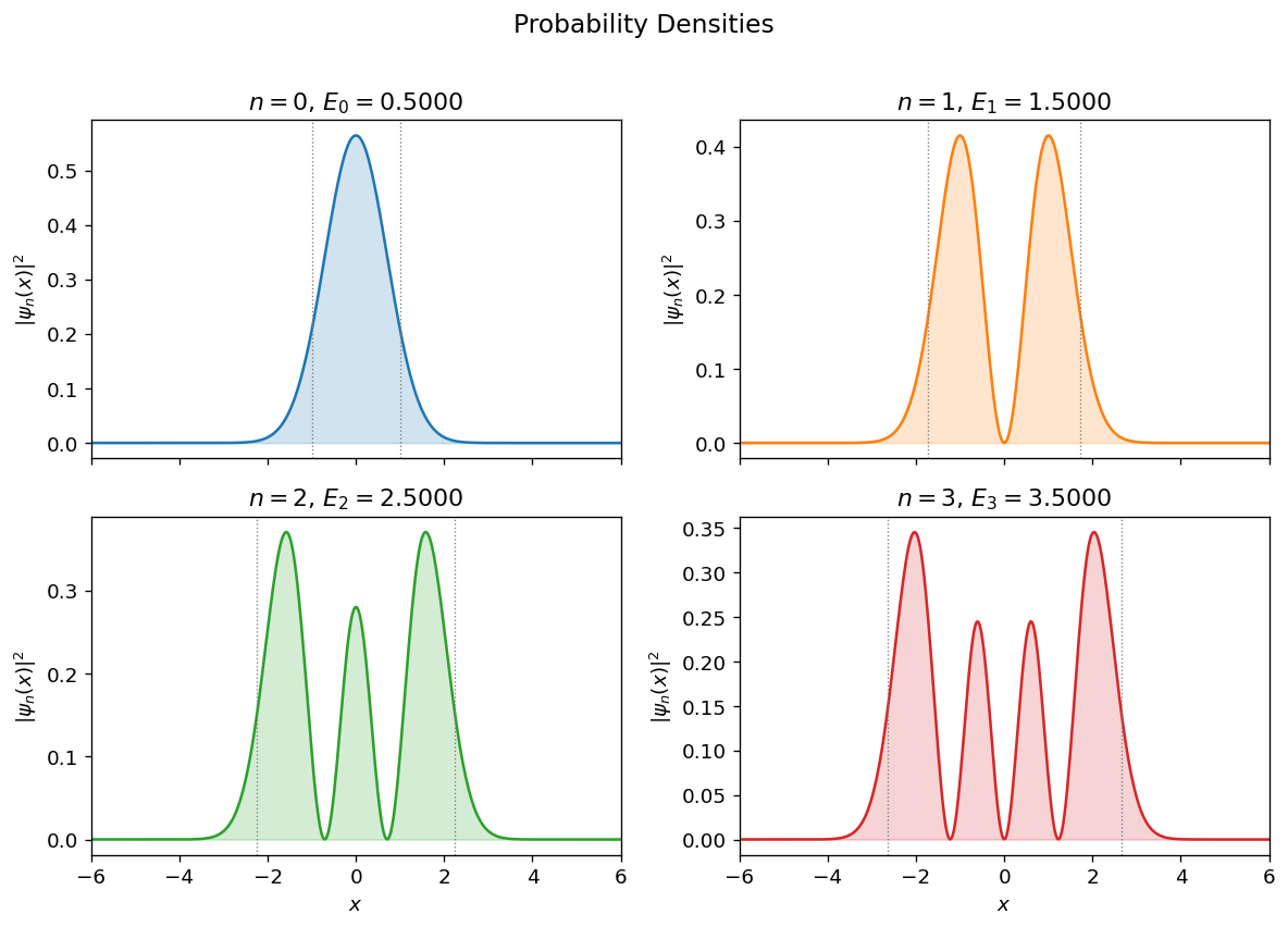
Probability densities

Plot \(|\psi_n(x)|^2\) for the first four eigenstates in a 2x2 subplot grid.

fig, axes = plt.subplots(2, 2, figsize=(10, 7), sharex=True)

for n, ax in enumerate(axes.flat):
    psi = eigvecs[:, n].real

    # Interpolate onto fine grid
    psi_fine = CubicSpline(x_sorted, psi[sort_idx])(x_fine)
    prob_fine = psi_fine**2

    color = colors[n % len(colors)]
    ax.plot(x_fine, prob_fine, color=color, linewidth=1.5)
    ax.fill_between(x_fine, prob_fine, alpha=0.2, color=color)

    # Mark classical turning points: V(x_tp) = E_n => x_tp = +/- sqrt(2*E_n)
    E_n = eigvals[n]
    x_tp = np.sqrt(2 * E_n)
    ax.axvline(x_tp, color="gray", linestyle=":", linewidth=0.8)
    ax.axvline(-x_tp, color="gray", linestyle=":", linewidth=0.8)

    ax.set_xlim(-6, 6)
    ax.set_title(f"$n = {n}$, $E_{n} = {E_n:.4f}$")
    ax.set_ylabel("$|\\psi_n(x)|^2$")

for ax in axes[1]:
    ax.set_xlabel("$x$")

fig.suptitle("Probability Densities", fontsize=14, y=1.01)
plt.tight_layout()
plt.show()

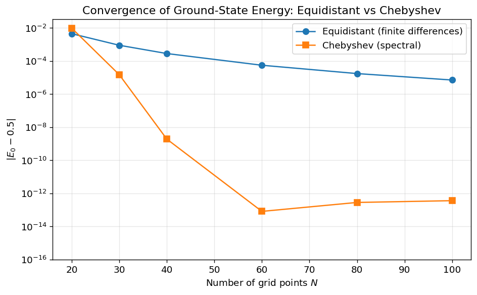
Convergence study: Equidistant vs Chebyshev

We now compare the convergence of the ground-state energy \(E_0\) as a function of the number of grid points \(N\) for both equidistant (finite difference) and Chebyshev (spectral) grids.

The key prediction from numerical analysis:

• Equidistant grids with finite differences converge algebraically (polynomial in \(N\)).

• Chebyshev grids with spectral differentiation converge exponentially (straight line on a semilog plot).

def compute_ground_state_energy(axis_type, N, L=8.0):
    """Compute the ground-state energy E_0 for a given grid type and resolution."""
    grid = Grid(create_axis(axis_type, N, -L, L))
    x = grid.coords

    T = -0.5 * Diff(grid, 2, 0).as_matrix()
    V = scipy.sparse.diags(0.5 * x**2)
    H = (T + V).tocsc()

    # Extract interior submatrix (Dirichlet BCs: psi=0 at boundaries)
    interior = np.arange(1, grid.size - 1)
    H_int = H[np.ix_(interior, interior)].tocsc()

    # Get a few smallest eigenvalues
    eigvals, _ = eigs(H_int, k=4, which="SR")
    eigvals = np.sort(eigvals.real)

    return eigvals[0]

N_values = [20, 30, 40, 60, 80, 100]
E0_exact = 0.5

errors_equidistant = []
errors_chebyshev = []

print(f"{'N':>5s}  {'Equidistant E0':>16s}  {'Error':>12s}  {'Chebyshev E0':>16s}  {'Error':>12s}")
print("-" * 70)

for N in N_values:
    E0_equi = compute_ground_state_energy(AxisType.EQUIDISTANT, N)
    E0_cheb = compute_ground_state_energy(AxisType.CHEBYSHEV, N)

    err_equi = abs(E0_equi - E0_exact)
    err_cheb = abs(E0_cheb - E0_exact)

    errors_equidistant.append(err_equi)
    errors_chebyshev.append(err_cheb)

    print(f"{N:5d}  {E0_equi:16.12f}  {err_equi:12.2e}  {E0_cheb:16.12f}  {err_cheb:12.2e}")

    N    Equidistant E0         Error      Chebyshev E0         Error
----------------------------------------------------------------------
   20    0.495541136789      4.46e-03    0.509629033051      9.63e-03
   30    0.499110060588      8.90e-04    0.500014810761      1.48e-05
   40    0.499718750379      2.81e-04    0.500000001895      1.89e-09
   60    0.499944891332      5.51e-05    0.500000000000      8.07e-14
   80    0.499982691462      1.73e-05    0.500000000000      2.80e-13
  100    0.499992950229      7.05e-06    0.500000000000      3.59e-13

fig, ax = plt.subplots(figsize=(8, 5))

ax.semilogy(N_values, errors_equidistant, "o-", color="C0", linewidth=1.5,
            markersize=7, label="Equidistant (finite differences)")
ax.semilogy(N_values, errors_chebyshev, "s-", color="C1", linewidth=1.5,
            markersize=7, label="Chebyshev (spectral)")

ax.set_xlabel("Number of grid points $N$")
ax.set_ylabel("$|E_0 - 0.5|$")
ax.set_title("Convergence of Ground-State Energy: Equidistant vs Chebyshev")
ax.legend(fontsize=11)
ax.grid(True, which="both", alpha=0.3)
ax.set_ylim(bottom=1e-16)

plt.tight_layout()
plt.show()

Summary

• The Chebyshev spectral method achieves exponential convergence: the error drops as a straight line on the semilog plot, reaching machine precision with relatively few grid points.

• The equidistant finite-difference method converges only algebraically (polynomial rate), requiring far more grid points to reach comparable accuracy.

• For smooth problems like the quantum harmonic oscillator, spectral methods are vastly more efficient than finite differences. The numgrids library makes it easy to switch between discretization strategies by simply changing the axis type.