Heat Diffusion in a Rod

This notebook solves the classical 1D heat equation on a rod of unit length using numgrids.

The heat equation describes how temperature \(u(x, t)\) evolves over time due to thermal diffusion:

\[\frac{\partial u}{\partial t} = \kappa \, \frac{\partial^2 u}{\partial x^2}, \qquad x \in [0, 1]\]

where \(\kappa = 0.01\) is the thermal diffusivity.

Boundary conditions: The rod is held at zero temperature at both ends (Dirichlet):

\[u(0, t) = 0, \qquad u(1, t) = 0\]

Initial condition: A sinusoidal temperature profile:

\[u(x, 0) = \sin(\pi x)\]

This problem has the exact analytical solution:

\[u(x, t) = \sin(\pi x) \, e^{-\kappa \pi^2 t}\]

which makes it an ideal test case for validating the numerical method.

Setup: Grid and Differential Operator

We begin by creating an equidistant 1D grid with 80 points on \([0, 1]\) and constructing the sparse matrix representation of the second-derivative (Laplacian) operator \(\partial^2 / \partial x^2\).

import numpy as np
import matplotlib.pyplot as plt
from numgrids import *

plt.style.use('default')

# Physical parameters
kappa = 0.01  # thermal diffusivity

# Create a 1D equidistant grid on [0, 1]
axis = create_axis(AxisType.EQUIDISTANT, 80, 0, 1)
grid = Grid(axis)
x = grid.coords

print(f"Grid: {grid}")
print(f"Number of points: {len(x)}")
print(f"Grid spacing dx = {x[1] - x[0]:.6f}")

Grid: Grid(shape=(80,), ndims=1)
Number of points: 80
Grid spacing dx = 0.012658

# Build the sparse Laplacian matrix
D2 = Diff(grid, 2, 0)
L = D2.as_matrix()

print(f"Laplacian matrix: {L}")

Laplacian matrix: <Compressed Sparse Row sparse matrix of dtype 'float64'
        with 404 stored elements and shape (80, 80)>
  Coords        Values
  (0, 0)        23403.749999999713
  (0, 1)        -80092.83333333224
  (0, 2)        111297.83333333164
  (0, 3)        -81132.99999999868
  (0, 4)        31725.0833333328
  (0, 5)        -5200.833333333244
  (1, 1)        23403.749999999713
  (1, 2)        -80092.83333333224
  (1, 3)        111297.83333333164
  (1, 4)        -81132.99999999868
  (1, 5)        31725.0833333328
  (1, 6)        -5200.833333333244
  (2, 0)        -520.0833333333331
  (2, 1)        8321.33333333333
  (2, 2)        -15602.499999999998
  (2, 3)        8321.333333333334
  (2, 4)        -520.0833333333334
  (3, 1)        -520.0833333333331
  (3, 2)        8321.33333333333
  (3, 3)        -15602.499999999998
  (3, 4)        8321.333333333334
  (3, 5)        -520.0833333333334
  (4, 2)        -520.0833333333331
  (4, 3)        8321.33333333333
  (4, 4)        -15602.499999999998
  :     :
  (75, 75)      -15602.499999999998
  (75, 76)      8321.333333333334
  (75, 77)      -520.0833333333334
  (76, 74)      -520.0833333333331
  (76, 75)      8321.33333333333
  (76, 76)      -15602.499999999998
  (76, 77)      8321.333333333334
  (76, 78)      -520.0833333333334
  (77, 75)      -520.0833333333331
  (77, 76)      8321.33333333333
  (77, 77)      -15602.499999999998
  (77, 78)      8321.333333333334
  (77, 79)      -520.0833333333334
  (78, 73)      -5200.833333333423
  (78, 74)      31725.083333333852
  (78, 75)      -81133.00000000124
  (78, 76)      111297.83333333481
  (78, 77)      -80092.83333333423
  (78, 78)      23403.75000000022
  (79, 74)      -5200.833333333423
  (79, 75)      31725.083333333852
  (79, 76)      -81133.00000000124
  (79, 77)      111297.83333333481
  (79, 78)      -80092.83333333423
  (79, 79)      23403.75000000022

Boundary Conditions

We set up Dirichlet boundary conditions \(u = 0\) at both ends of the rod. At each time step we enforce these by calling DirichletBC.apply(u) on the solution array, which directly sets the boundary values to zero.

# Define boundary faces and Dirichlet conditions
face_left = grid.faces["0_low"]
face_right = grid.faces["0_high"]

bc_left = DirichletBC(face_left, 0.0)
bc_right = DirichletBC(face_right, 0.0)

print(f"Left face:  {face_left}")
print(f"Right face: {face_right}")

Left face:  BoundaryFace(axis=0, side='low')
Right face: BoundaryFace(axis=0, side='high')

Time Integration with Explicit Euler

We discretize in time using the forward Euler method:

\[u^{n+1} = u^n + \Delta t \, \kappa \, L \, u^n\]

where \(L\) is the sparse Laplacian matrix. The CFL stability condition for the explicit scheme requires \(\Delta t \leq \Delta x^2 / (2\kappa)\). We use a safety factor of 0.4 to stay well within the stable regime:

\[\Delta t = 0.4 \, \frac{\Delta x^2}{\kappa}\]

We run for 200 time steps and save a snapshot every 20 steps.

# Initial condition
u = np.sin(np.pi * x)

# Time-stepping parameters
dx = x[1] - x[0]
dt = 0.4 * dx**2 / kappa  # stability condition
n_steps = 200
save_every = 20

print(f"dt = {dt:.6e}")
print(f"Total simulation time = {n_steps * dt:.4f}")
print(f"CFL number (kappa * dt / dx^2) = {kappa * dt / dx**2:.2f}")

# Storage for snapshots
snapshots = [u.copy()]
times = [0.0]

# Explicit Euler time-stepping loop
t = 0.0
for step in range(1, n_steps + 1):
    u = u + dt * kappa * (L @ u)
    bc_left.apply(u)
    bc_right.apply(u)
    t += dt

    if step % save_every == 0:
        snapshots.append(u.copy())
        times.append(t)

print(f"\nCompleted {n_steps} time steps.")
print(f"Saved {len(snapshots)} snapshots (including t=0).")
print(f"Final time: t = {times[-1]:.4f}")

dt = 6.409229e-03
Total simulation time = 1.2818
CFL number (kappa * dt / dx^2) = 0.40

Completed 200 time steps.
Saved 11 snapshots (including t=0).
Final time: t = 1.2818

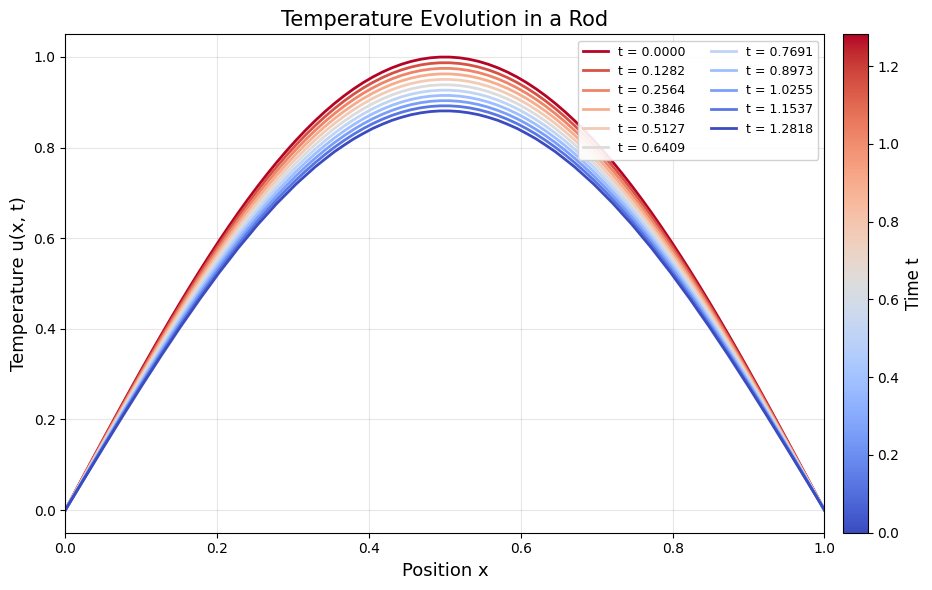
Plot 1: Waterfall Plot of Temperature Profiles

Each curve shows the temperature distribution \(u(x)\) at a different time. Lines are colored from hot (red) at \(t = 0\) to cold (blue) at the final time, reflecting the physical cooling of the rod.

fig, ax = plt.subplots(figsize=(10, 6))

cmap = plt.cm.coolwarm
n_snaps = len(snapshots)

for i, (snap, t_snap) in enumerate(zip(snapshots, times)):
    color = cmap(1.0 - i / (n_snaps - 1))  # red (hot) -> blue (cold)
    ax.plot(x, snap, color=color, linewidth=2, label=f"t = {t_snap:.4f}")

ax.set_xlabel("Position x", fontsize=13)
ax.set_ylabel("Temperature u(x, t)", fontsize=13)
ax.set_title("Temperature Evolution in a Rod", fontsize=15)
ax.legend(loc="upper right", fontsize=9, ncol=2, framealpha=0.9)
ax.set_xlim(0, 1)
ax.set_ylim(-0.05, 1.05)
ax.grid(True, alpha=0.3)

# Add a colorbar to indicate time
sm = plt.cm.ScalarMappable(cmap=cmap, norm=plt.Normalize(vmin=times[0], vmax=times[-1]))
sm.set_array([])
cbar = fig.colorbar(sm, ax=ax, pad=0.02)
cbar.set_label("Time t", fontsize=12)

fig.tight_layout()
plt.show()

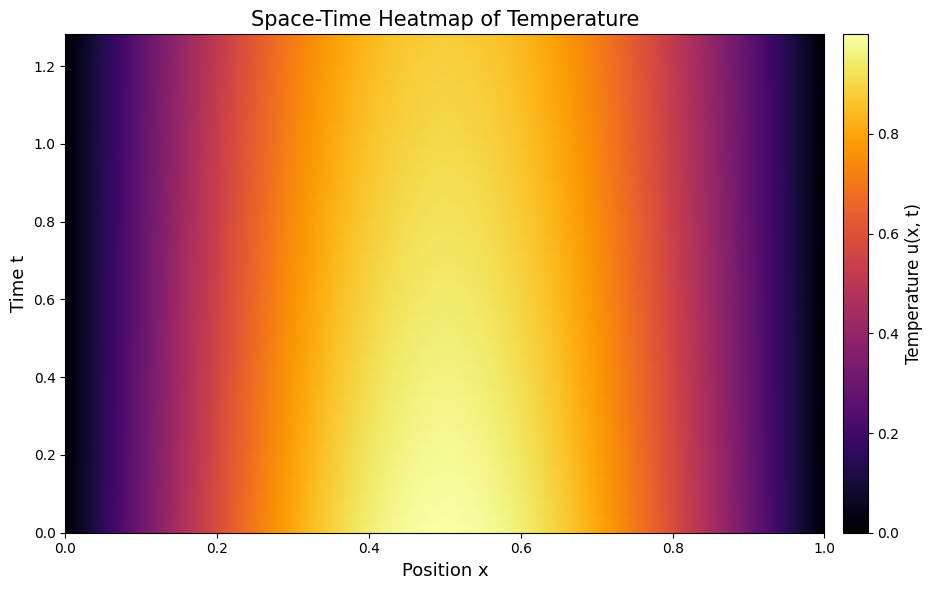
Plot 2: Space-Time Heatmap

A filled contour plot showing the complete temperature evolution \(u(x, t)\) as a heatmap. The horizontal axis is position, the vertical axis is time, and color intensity represents temperature.

# Re-run the simulation, saving every step for a smooth heatmap
u_heatmap = np.sin(np.pi * x)
all_u = [u_heatmap.copy()]
all_t = [0.0]

t = 0.0
for step in range(1, n_steps + 1):
    u_heatmap = u_heatmap + dt * kappa * (L @ u_heatmap)
    bc_left.apply(u_heatmap)
    bc_right.apply(u_heatmap)
    t += dt
    all_u.append(u_heatmap.copy())
    all_t.append(t)

# Assemble into a 2D array: rows = time, columns = space
U = np.array(all_u)
T_arr = np.array(all_t)

fig, ax = plt.subplots(figsize=(10, 6))

X_mesh, T_mesh = np.meshgrid(x, T_arr)
pcm = ax.pcolormesh(X_mesh, T_mesh, U, cmap="inferno", shading="gouraud")

ax.set_xlabel("Position x", fontsize=13)
ax.set_ylabel("Time t", fontsize=13)
ax.set_title("Space-Time Heatmap of Temperature", fontsize=15)

cbar = fig.colorbar(pcm, ax=ax, pad=0.02)
cbar.set_label("Temperature u(x, t)", fontsize=12)

fig.tight_layout()
plt.show()

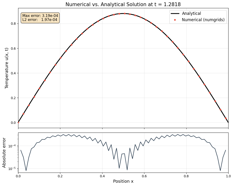
Plot 3: Numerical vs. Analytical Solution

We compare the numerical solution at the final time step with the exact analytical solution \(u(x, t) = \sin(\pi x) \, e^{-\kappa \pi^2 t}\) to assess the accuracy of the scheme.

# Analytical solution at final time
t_final = times[-1]
u_exact = np.sin(np.pi * x) * np.exp(-kappa * np.pi**2 * t_final)
u_numerical = snapshots[-1]

# Compute errors
error = np.abs(u_numerical - u_exact)
max_error = np.max(error)
l2_error = np.sqrt(np.mean(error**2))

fig, (ax1, ax2) = plt.subplots(2, 1, figsize=(10, 8), height_ratios=[3, 1], sharex=True)

# Top panel: solution comparison
ax1.plot(x, u_exact, 'k-', linewidth=2.5, label='Analytical')
ax1.plot(x, u_numerical, 'o', color='#e74c3c', markersize=4, markevery=2,
         label='Numerical (numgrids)', zorder=5)
ax1.set_ylabel("Temperature u(x, t)", fontsize=13)
ax1.set_title(f"Numerical vs. Analytical Solution at t = {t_final:.4f}", fontsize=15)
ax1.legend(fontsize=12)
ax1.grid(True, alpha=0.3)

# Annotate the error
ax1.annotate(
    f"Max error: {max_error:.2e}\nL2 error:   {l2_error:.2e}",
    xy=(0.02, 0.95), xycoords='axes fraction',
    fontsize=11, verticalalignment='top',
    bbox=dict(boxstyle='round,pad=0.4', facecolor='wheat', alpha=0.8)
)

# Bottom panel: pointwise error
ax2.semilogy(x[1:-1], error[1:-1], '-', color='#2c3e50', linewidth=1.5)
ax2.set_xlabel("Position x", fontsize=13)
ax2.set_ylabel("Absolute error", fontsize=13)
ax2.grid(True, alpha=0.3)
ax2.set_xlim(0, 1)

fig.tight_layout()
plt.show()

Summary

In this notebook we demonstrated how to solve the 1D heat equation using numgrids:

1. We created a 1D equidistant grid and used Diff(grid, 2, 0).as_matrix() to obtain a sparse Laplacian matrix.

2. We applied homogeneous Dirichlet boundary conditions at each time step via DirichletBC.apply().

3. We time-stepped the solution using explicit (forward) Euler with a CFL-stable time step.

4. The waterfall plot showed the progressive cooling of the rod from its initial sinusoidal temperature profile toward thermal equilibrium at \(u = 0\).

5. The space-time heatmap gave a global view of the diffusion process.

6. The comparison plot confirmed that the numerical solution closely matches the analytical result, with the pointwise error remaining small throughout the domain.

The combination of numgrids’ sparse differential operators with a simple explicit time-stepper provides an efficient and accurate solver for parabolic PDEs.