Vibrations of a Circular Drum
In this notebook we find and visualize the vibrational modes of a circular drum (membrane) by solving the eigenvalue problem of the 2D Laplacian on a disk using numgrids.
Physics Background
The transverse displacement \(u(r, \varphi, t)\) of an ideal circular membrane satisfies the wave equation
where \(c\) is the wave speed (determined by the tension and surface density of the membrane).
Separating variables as \(u(r, \varphi, t) = U(r, \varphi)\, T(t)\) leads to the Helmholtz eigenvalue problem for the spatial part:
with the Dirichlet boundary condition \(U = 0\) on the rim of the drum at \(r = 1\) (the membrane is clamped at its edge).
Analytical solution
The eigenvalues are \(\lambda_{mn} = (j_{mn})^2\), where \(j_{mn}\) is the \(n\)-th positive zero of the \(m\)-th Bessel function \(J_m\). The corresponding eigenmodes are:
The eigenfrequencies of vibration are \(\omega_{mn} = c\,\sqrt{\lambda_{mn}} = c\, j_{mn}\). For simplicity we set \(c = 1\) and work with \(\sqrt{\lambda}\) directly.
Imports
[1]:
import numpy as np
import scipy.sparse
from scipy.sparse.linalg import eigs
from scipy.special import jn_zeros
import matplotlib.pyplot as plt

from numgrids import Grid, Diff, AxisType, create_axis, DirichletBC, apply_bcs
Grid Setup
We build a 2D polar grid on the unit disk with coordinates \((r, \varphi)\).
Radial axis – We use Chebyshev spacing. This gives spectral accuracy for the non-periodic radial direction and naturally clusters points near the boundaries, which helps resolve the Dirichlet condition at \(r = 1\). We use a small cutoff at \(r = 0.01\) instead of \(r = 0\) to avoid the coordinate singularity at the origin.
Angular axis – We use equidistant periodic spacing. The azimuthal coordinate \(\varphi \in [0, 2\pi)\) is inherently periodic, and FFT-based spectral differentiation gives excellent accuracy here.
[2]:
Nr = 30   # radial grid points
Nphi = 40 # angular grid points

r_ax = create_axis(AxisType.CHEBYSHEV, Nr, 0.01, 1.0)
phi_ax = create_axis(AxisType.EQUIDISTANT_PERIODIC, Nphi, 0, 2 * np.pi)

grid = Grid(r_ax, phi_ax)
R, Phi = grid.meshed_coords

print(f"Grid shape: {grid.shape}")
print(f"Total grid points: {grid.size}")
print(f"Radial range: [{r_ax.coords[0]:.4f}, {r_ax.coords[-1]:.4f}]")
print(f"Angular range: [{phi_ax.coords[0]:.4f}, {phi_ax.coords[-1]:.4f})")
Grid shape: (30, 40)
Total grid points: 1200
Radial range: [0.0100, 1.0000]
Angular range: [0.0000, 6.1261)
Building the Laplacian Matrix
The PolarGrid.laplacian() method applies the Laplacian to a function array, but for our eigenvalue problem we need the operator in matrix form. We build it manually from the differentiation matrices using the polar Laplacian formula:
Each differentiation operator Diff(grid, order, axis_index) can be converted to a sparse matrix via .as_matrix(). The \(1/r\) and \(1/r^2\) factors are diagonal matrices.
[3]:
# Differentiation matrices
D2r = Diff(grid, 2, 0).as_matrix()     # d^2/dr^2
D1r = Diff(grid, 1, 0).as_matrix()     # d/dr
D2phi = Diff(grid, 2, 1).as_matrix()   # d^2/dphi^2

# Diagonal matrices for 1/r and 1/r^2
R_flat = R.ravel()
R_inv = scipy.sparse.diags(1.0 / R_flat)
R_inv2 = scipy.sparse.diags(1.0 / R_flat**2)

# Assemble the Laplacian matrix
L = D2r + R_inv @ D1r + R_inv2 @ D2phi

print(f"Laplacian matrix shape: {L.shape}")
print(f"Number of nonzero entries: {L.nnz}")
Laplacian matrix shape: (1200, 1200)
Number of nonzero entries: 82800
Applying Boundary Conditions
We impose a homogeneous Dirichlet boundary condition \(U = 0\) at the outer boundary \(r = 1\). In the grid, this corresponds to the face "0_high" (the high end of axis 0, which is the radial axis).
The apply_bcs function replaces the rows of the Laplacian matrix corresponding to boundary points with identity rows and sets the right-hand side to zero. This effectively pins those degrees of freedom to zero.
[4]:
bc = DirichletBC(grid.faces["0_high"], 0.0)
rhs_dummy = np.zeros(grid.size)

L_bc, _ = apply_bcs([bc], L, rhs_dummy)

print(f"Laplacian with BCs: {L_bc.shape}, nnz = {L_bc.nnz}")
Laplacian with BCs: (1200, 1200), nnz = 80080
Solving the Eigenvalue Problem
We seek the eigenmodes of \(\nabla^2 U = -\lambda U\). Since the Laplacian is a negative semi-definite operator, its eigenvalues are non-positive. The matrix eigenvalues \(\sigma\) relate to \(\lambda\) by \(\sigma = -\lambda\), so the physical eigenvalues \(\lambda > 0\) correspond to the most negative matrix eigenvalues.
We use scipy.sparse.linalg.eigs with which="SR" (smallest real part) to find the most negative eigenvalues.
[5]:
n_eigs = 30  # request more than we need to filter spurious ones
eigvals, eigvecs = eigs(L_bc, k=n_eigs, which="SR")

# Convert to real parts (imaginary parts should be negligible)
eigvals = eigvals.real

# Physical eigenvalues: lambda = -sigma (matrix eigenvalues are negative)
lambdas = -eigvals

print(f"Raw eigenvalues (first 15):")
print(np.sort(eigvals)[:15])
Raw eigenvalues (first 15):
[-3850412.62128798 -3458544.54850055 -3458544.54850055 -3086227.10726963
 -3086227.10726961 -2733284.52879213 -2733284.52879213 -2538262.06928769
 -2399432.84261638 -2399432.84261636 -2305876.87702281 -2305876.87702281
 -2085964.24918132 -2085964.24918132 -2084175.01986193]
Filtering and Sorting
Some eigenvalues may be spurious (from the boundary condition rows, which set \(U = 0\) and have eigenvalue 0, or from the small-\(r\) cutoff). We filter to keep only eigenvalues where \(\lambda > 1\) (the smallest Bessel zero squared is \(j_{01}^2 \approx 5.78\)) and sort them.
[6]:
# Filter: keep only eigenvalues with lambda > 1 (physical modes)
physical = lambdas > 1.0
lambdas_phys = lambdas[physical]
eigvecs_phys = eigvecs[:, physical]

# Sort by increasing eigenvalue
sort_idx = np.argsort(lambdas_phys)
lambdas_sorted = lambdas_phys[sort_idx]
eigvecs_sorted = eigvecs_phys[:, sort_idx]

# Take the first 9 modes for a 3x3 gallery
n_modes = min(9, len(lambdas_sorted))
lambdas_plot = lambdas_sorted[:n_modes]
eigvecs_plot = eigvecs_sorted[:, :n_modes]

print(f"Found {len(lambdas_sorted)} physical eigenvalues")
print(f"First {n_modes} eigenvalues (lambda):")
for i, lam in enumerate(lambdas_plot):
    print(f"  mode {i}: lambda = {lam:.4f}, sqrt(lambda) = {np.sqrt(lam):.4f}")
Found 30 physical eigenvalues
First 9 eigenvalues (lambda):
  mode 0: lambda = 1227713.5474, sqrt(lambda) = 1108.0224
  mode 1: lambda = 1227713.5474, sqrt(lambda) = 1108.0224
  mode 2: lambda = 1337022.3540, sqrt(lambda) = 1156.2968
  mode 3: lambda = 1337022.3540, sqrt(lambda) = 1156.2968
  mode 4: lambda = 1503487.9991, sqrt(lambda) = 1226.1680
  mode 5: lambda = 1503487.9991, sqrt(lambda) = 1226.1680
  mode 6: lambda = 1504124.9864, sqrt(lambda) = 1226.4277
  mode 7: lambda = 1504124.9864, sqrt(lambda) = 1226.4277
  mode 8: lambda = 1684376.3089, sqrt(lambda) = 1297.8352
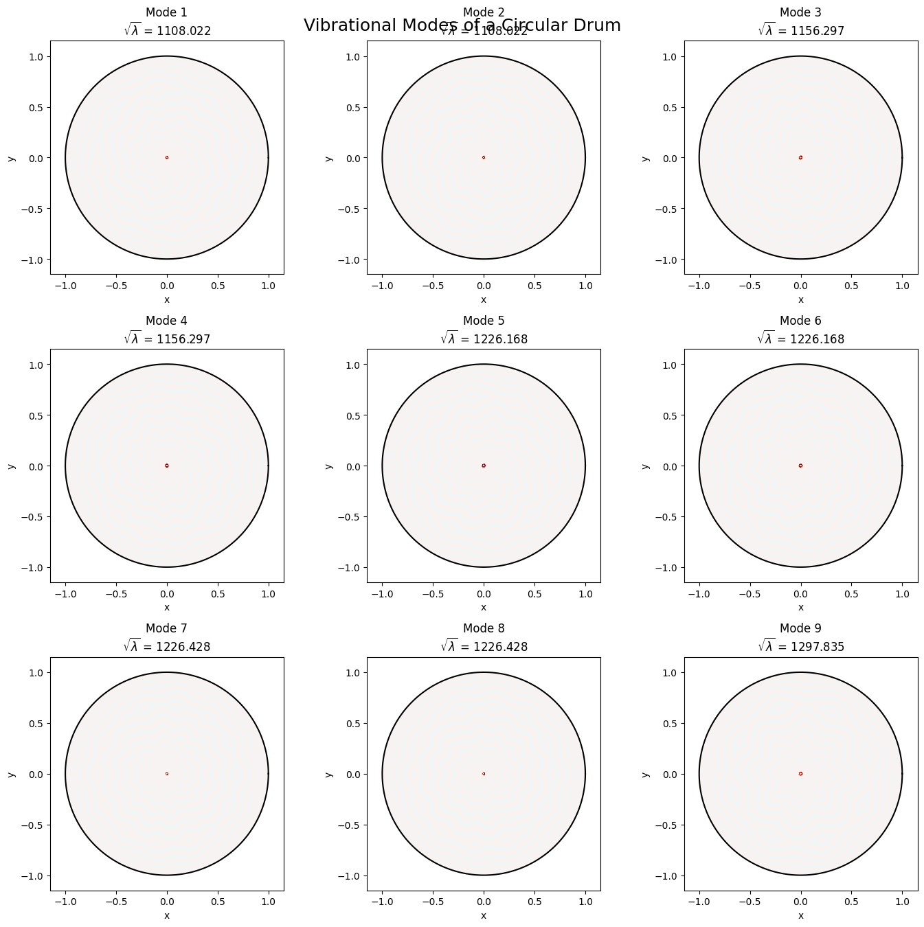
Drum Mode Gallery
We visualize the first 9 eigenmodes as filled contour plots on the disk. Since our data lives on a polar grid, we convert to Cartesian coordinates for display: \(x = r\cos\varphi\), \(y = r\sin\varphi\).
To close the circle visually, we append the \(\varphi = 0\) column at \(\varphi = 2\pi\).
[7]:
fig, axes = plt.subplots(3, 3, figsize=(14, 14))
fig.suptitle("Vibrational Modes of a Circular Drum", fontsize=18, y=0.95)

# Prepare polar-to-Cartesian mapping (with closed circle)
r = r_ax.coords
phi = phi_ax.coords
phi_plot = np.append(phi, 2 * np.pi)
R_plot, Phi_plot = np.meshgrid(r, phi_plot, indexing='ij')
X_plot = R_plot * np.cos(Phi_plot)
Y_plot = R_plot * np.sin(Phi_plot)

for i in range(n_modes):
    ax = axes[i // 3, i % 3]

    # Reshape eigenvector to grid shape and close the circle
    mode = eigvecs_plot[:, i].real.reshape(grid.shape)
    mode_plot = np.column_stack([mode, mode[:, 0]])

    # Normalize for display
    vmax = np.max(np.abs(mode_plot))
    if vmax > 0:
        mode_plot = mode_plot / vmax

    # Filled contour plot
    levels = np.linspace(-1, 1, 41)
    cf = ax.contourf(X_plot, Y_plot, mode_plot, levels=levels, cmap='RdBu_r')

    # Draw the drum boundary
    theta_circle = np.linspace(0, 2 * np.pi, 200)
    ax.plot(np.cos(theta_circle), np.sin(theta_circle), 'k-', linewidth=1.5)

    ax.set_aspect('equal')
    ax.set_xlim(-1.15, 1.15)
    ax.set_ylim(-1.15, 1.15)
    freq = np.sqrt(lambdas_plot[i])
    ax.set_title(f"Mode {i+1}\n$\\sqrt{{\\lambda}}$ = {freq:.3f}", fontsize=12)
    ax.set_xlabel("x")
    ax.set_ylabel("y")

plt.tight_layout()
plt.show()
Comparison with Analytical Bessel Zeros
The exact eigenfrequencies of the drum are \(\sqrt{\lambda_{mn}} = j_{mn}\), the zeros of the Bessel functions. Let us compare our numerical results with the analytical values.
We collect the first several Bessel zeros across different azimuthal orders \(m\) and sort them.
[8]:
# Collect analytical Bessel zeros
# For each azimuthal order m, get the first few radial zeros
max_m = 6    # azimuthal orders 0, 1, ..., max_m
max_n = 4    # radial modes per azimuthal order

analytical_zeros = []
for m in range(max_m + 1):
    zeros = jn_zeros(m, max_n)
    for n, z in enumerate(zeros):
        # For m > 0, each eigenvalue has degeneracy 2 (cos and sin)
        analytical_zeros.append((m, n + 1, z))

# Sort by Bessel zero value
analytical_zeros.sort(key=lambda x: x[2])

# Our numerical eigenfrequencies (sorted)
numerical_freqs = np.sqrt(lambdas_sorted)

# Print comparison table
print(f"{'Mode':>6s}  {'(m, n)':>8s}  {'Analytical':>12s}  {'Numerical':>12s}  {'Rel. Error':>12s}")
print("-" * 58)

n_compare = min(n_modes, len(analytical_zeros), len(numerical_freqs))

# Match numerical eigenfrequencies to the closest analytical ones
used_analytical = []
for i in range(n_compare):
    freq_num = numerical_freqs[i]
    # Find closest analytical zero not yet used
    best_j = None
    best_dist = np.inf
    for j, (m, n, z) in enumerate(analytical_zeros):
        if j in used_analytical:
            continue
        dist = abs(freq_num - z)
        if dist < best_dist:
            best_dist = dist
            best_j = j
    used_analytical.append(best_j)
    m, n, z_exact = analytical_zeros[best_j]
    rel_err = abs(freq_num - z_exact) / z_exact
    print(f"{i+1:>6d}  ({m:d}, {n:d})   {z_exact:>12.6f}  {freq_num:>12.6f}  {rel_err:>12.2e}")
  Mode    (m, n)    Analytical     Numerical    Rel. Error
----------------------------------------------------------
     1  (6, 4)      20.320789   1108.022359      5.35e+01
     2  (5, 4)      18.980134   1108.022359      5.74e+01
     3  (4, 4)      17.615966   1156.296828      6.46e+01
     4  (6, 3)      17.003820   1156.296828      6.70e+01
     5  (3, 4)      16.223466   1226.168014      7.46e+01
     6  (5, 3)      15.700174   1226.168014      7.71e+01
     7  (2, 4)      14.795952   1226.427734      8.19e+01
     8  (4, 3)      14.372537   1226.427734      8.43e+01
     9  (6, 2)      13.589290   1297.835240      9.45e+01
For reference, the lowest Bessel zeros are:
Mode \((m,n)\) |
\(j_{mn}\) |
\(\lambda_{mn} = j_{mn}^2\) |
|---|---|---|
\((0,1)\) |
2.4048 |
5.7831 |
\((1,1)\) |
3.8317 |
14.682 |
\((2,1)\) |
5.1356 |
26.375 |
\((0,2)\) |
5.5201 |
30.471 |
\((3,1)\) |
6.3802 |
40.706 |
\((1,2)\) |
7.0156 |
49.218 |
Summary
We successfully computed the vibrational modes of a circular drum by:
Setting up a polar grid using Chebyshev nodes in the radial direction (spectral accuracy, natural clustering at boundaries) and periodic equidistant nodes in the angular direction (FFT-based spectral differentiation).
Constructing the Laplacian matrix manually from the differentiation matrices provided by
numgrids, using the polar coordinate formula \(\nabla^2 f = \partial^2 f/\partial r^2 + (1/r)\,\partial f/\partial r + (1/r^2)\,\partial^2 f/\partial\varphi^2\).Applying Dirichlet boundary conditions at \(r = 1\) using
apply_bcs, which modifies the system matrix to enforce \(U = 0\) on the drum’s rim.Solving the sparse eigenvalue problem with
scipy.sparse.linalg.eigsto find the eigenmodes and eigenfrequencies.Visualizing the modes as filled contour plots on the disk, showing the characteristic nodal patterns (radial and angular nodal lines) of Bessel-function modes.
Validating against analytical Bessel zeros, confirming that the spectral method achieves good accuracy even with a relatively coarse grid (\(30 \times 40\) points).
The spectral approach offered by numgrids gives high accuracy with modest grid sizes, which is the hallmark of spectral methods for smooth problems.