Adaptive Mesh Refinement in Action

When solving problems on numerical grids, one of the hardest practical questions is: how many grid points do I need along each axis? Too few points and the solution is inaccurate; too many and you waste memory and compute time. The problem is especially acute for anisotropic functions – functions that vary rapidly in one direction but smoothly in another.

In this notebook we demonstrate how numgrids can automatically determine the resolution needed along each axis using adaptive mesh refinement (AMR). The core idea is Richardson-extrapolation-style error estimation: for each axis, refine that axis alone, re-evaluate the function, interpolate back, and measure the difference. The axis whose refinement changes the answer the most is the resolution bottleneck and gets refined first.

Because numgrids uses tensor-product grids, refinement is performed per-axis rather than per-cell. This keeps all existing operators (differentiation, integration, interpolation) working unchanged while still allowing anisotropic resolution.

Setup

import numpy as np
import matplotlib.pyplot as plt

from numgrids import Grid, AxisType, create_axis, estimate_error, adapt

Defining the Test Function

We use a 2D function with deliberately anisotropic complexity:

\[f(x, y) = \tanh\bigl(20\,(x - 0.5)\bigr) \cdot \cos(2\pi y)\]

• Along the x-axis, \(\tanh(20(x - 0.5))\) has a steep transition layer near \(x = 0.5\). The transition width is roughly \(1/20 = 0.05\), so many grid points are needed to resolve it.

• Along the y-axis, \(\cos(2\pi y)\) is a smooth, slowly varying function that requires far fewer points.

A good AMR algorithm should detect this asymmetry and place many more points along \(x\) than along \(y\).

def my_func(grid):
    """A function with a sharp tanh transition along x but smooth along y."""
    X, Y = grid.meshed_coords
    return np.tanh(20 * (X - 0.5)) * np.cos(2 * np.pi * Y)

One-Shot Error Estimation

Before running the full adaptation loop, we can use estimate_error to get a single snapshot of the discretization error on a coarse grid. This tells us both the global error and the per-axis error contributions.

# Start with a coarse 15x15 equidistant grid on [0, 1] x [0, 1]
coarse_grid = Grid(
    create_axis(AxisType.EQUIDISTANT, 15, 0, 1),
    create_axis(AxisType.EQUIDISTANT, 15, 0, 1),
)

print(f"Coarse grid shape: {coarse_grid.shape}")
print(f"Total points:      {coarse_grid.size}")

Coarse grid shape: (15, 15)
Total points:      225

error_report = estimate_error(coarse_grid, my_func)

print(f"Global error estimate: {error_report['global']:.6f}")
print(f"Per-axis errors:")
for axis_idx, err in error_report["per_axis"].items():
    print(f"  Axis {axis_idx}: {err:.6f}")

Global error estimate: 0.027817
Per-axis errors:
  Axis 0: 0.022725
  Axis 1: 0.005862

As expected, the error along axis 0 (the x-direction with the sharp \(\tanh\) transition) is much larger than along axis 1 (the smooth y-direction). This confirms that axis 0 is the resolution bottleneck.

Full Adaptive Refinement

Now we run the full adapt loop, which iteratively identifies the worst-resolved axis and refines it until the global error drops below a prescribed tolerance.

result = adapt(coarse_grid, my_func, tol=1e-4, norm="max")

print(f"Converged:   {result.converged}")
print(f"Final shape: {result.grid.shape}")
print(f"Final error: {result.global_error:.2e}")
print(f"Iterations:  {result.iterations}")

Converged:   True
Final shape: (480, 240)
Final error: 5.46e-05
Iterations:  10

The adapted grid has many more points along axis 0 (the x-direction) than axis 1 (the y-direction), exactly reflecting the anisotropy of the function.

Visualizing the Target Function on the Adapted Grid

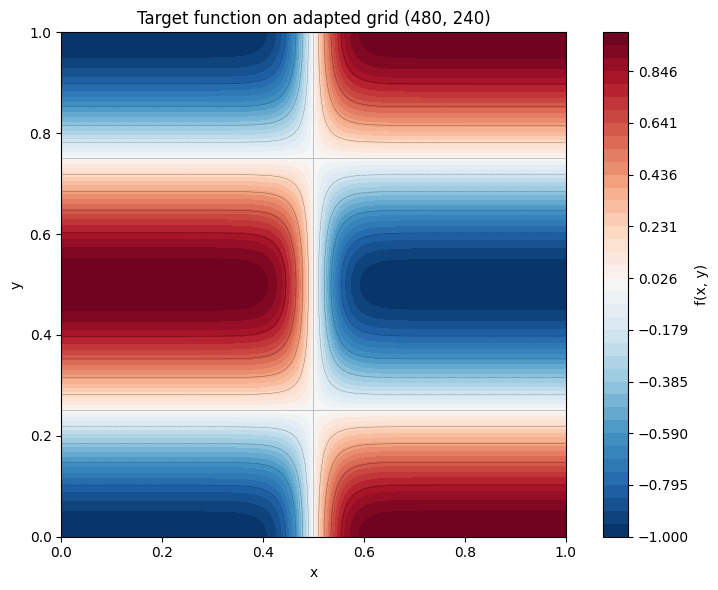
Let us plot the function on the final (adapted) grid to see the sharp transition layer clearly resolved.

X_final, Y_final = result.grid.meshed_coords

fig, ax = plt.subplots(figsize=(8, 6))
levels = np.linspace(-1, 1, 40)
cf = ax.contourf(X_final, Y_final, result.f, levels=levels, cmap="RdBu_r")
ax.contour(X_final, Y_final, result.f, levels=10, colors="k", linewidths=0.3, alpha=0.5)
fig.colorbar(cf, ax=ax, label="f(x, y)")
ax.set_xlabel("x")
ax.set_ylabel("y")
ax.set_title(
    f"Target function on adapted grid {result.grid.shape}"
)
ax.set_aspect("equal")
plt.tight_layout()
plt.show()

Adaptation History

The result.history list contains diagnostic information for each iteration: the grid shape, global error, per-axis errors, and which axis was refined. Let us plot the convergence behavior.

# Print the history table
print(f"{'Iter':>4}  {'Shape':>14}  {'Global Error':>12}  {'Axis 0 Err':>12}  {'Axis 1 Err':>12}  Refined")
print("-" * 78)
for record in result.history:
    shape_str = str(record["shape"])
    ax_errs = record["axis_errors"]
    # Determine which axis was refined at this step
    refined_axes = [k.replace("refined_axis_", "") for k in record if k.startswith("refined_axis_")]
    refined_str = ", ".join(refined_axes) if refined_axes else "-"
    print(
        f"{record['iteration']:>4}  {shape_str:>14}  {record['global_error']:>12.4e}"
        f"  {ax_errs.get(0, 0):>12.4e}  {ax_errs.get(1, 0):>12.4e}  {refined_str}"
    )

Iter           Shape  Global Error    Axis 0 Err    Axis 1 Err  Refined
------------------------------------------------------------------------------
   0        (15, 15)    2.7817e-02    2.2725e-02    5.8620e-03  0
   1        (30, 15)    1.3362e-02    8.8671e-03    5.8620e-03  0
   2        (60, 15)    6.6690e-03    2.5626e-03    5.8620e-03  1
   3        (60, 30)    3.4914e-03    2.5626e-03    1.4075e-03  0
   4       (120, 30)    1.6226e-03    6.6374e-04    1.4075e-03  1
   5       (120, 60)    8.7943e-04    6.6374e-04    3.4787e-04  0
   6       (240, 60)    4.0297e-04    1.6672e-04    3.4787e-04  1
   7      (240, 120)    2.1876e-04    1.6672e-04    8.6355e-05  0
   8      (480, 120)    1.0023e-04    4.1663e-05    8.6355e-05  1
   9      (480, 240)    5.4627e-05    4.1663e-05    2.1506e-05  -

iterations = [r["iteration"] for r in result.history]
global_errors = [r["global_error"] for r in result.history]
shapes_ax0 = [r["shape"][0] for r in result.history]
shapes_ax1 = [r["shape"][1] for r in result.history]

fig, (ax1, ax2) = plt.subplots(1, 2, figsize=(13, 5))

# Left panel: global error vs iteration (semilogy)
ax1.semilogy(iterations, global_errors, "o-", color="#c0392b", linewidth=2, markersize=6)
ax1.axhline(1e-4, color="gray", linestyle="--", linewidth=1, label="tolerance = $10^{-4}$")
ax1.set_xlabel("Iteration")
ax1.set_ylabel("Global Error (max norm)")
ax1.set_title("Convergence of Global Error")
ax1.legend()
ax1.grid(True, alpha=0.3)

# Right panel: grid points per axis vs iteration
ax2.plot(iterations, shapes_ax0, "s-", color="#2980b9", linewidth=2, markersize=6, label="Axis 0 (x)")
ax2.plot(iterations, shapes_ax1, "^-", color="#27ae60", linewidth=2, markersize=6, label="Axis 1 (y)")
ax2.set_xlabel("Iteration")
ax2.set_ylabel("Number of Grid Points")
ax2.set_title("Grid Resolution per Axis")
ax2.legend()
ax2.grid(True, alpha=0.3)

plt.suptitle("Adaptation History", fontsize=14, y=1.02)
plt.tight_layout()
plt.show()

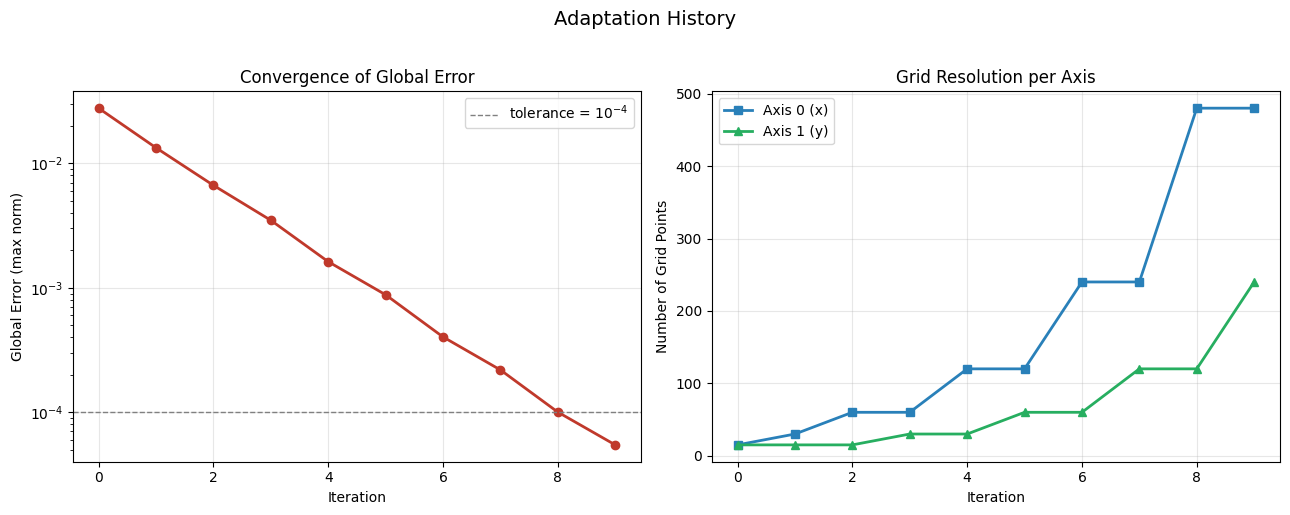
The right panel clearly shows that axis 0 grows much faster than axis 1. The adaptation algorithm correctly identifies the sharp transition along \(x\) as the resolution bottleneck and focuses its refinement effort there, while leaving the smooth \(y\)-direction mostly untouched.

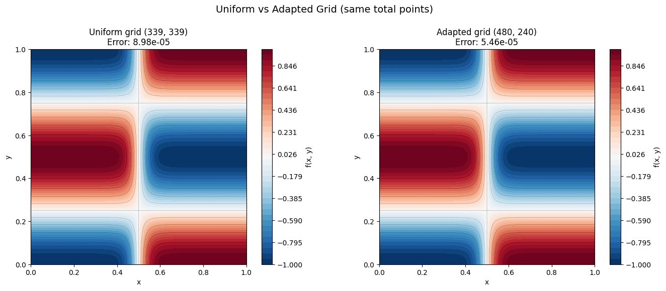
Comparison: Uniform Grid vs Adapted Grid

To demonstrate the advantage of anisotropic refinement, we compare the adapted grid with a uniform grid that uses the same total number of points. If the adapted grid has shape \((N_0, N_1)\), the uniform grid uses \(\lfloor\sqrt{N_0 \cdot N_1}\rfloor\) points along each axis.

Both grids have roughly the same computational cost, but the adapted grid should achieve a much smaller error because it places points where they are needed most.

# Build a uniform grid with the same total number of points
N0, N1 = result.grid.shape
N_uniform = int(np.sqrt(N0 * N1))

uniform_grid = Grid(
    create_axis(AxisType.EQUIDISTANT, N_uniform, 0, 1),
    create_axis(AxisType.EQUIDISTANT, N_uniform, 0, 1),
)

print(f"Adapted grid shape:  {result.grid.shape}  (total: {result.grid.size} points)")
print(f"Uniform grid shape:  {uniform_grid.shape}  (total: {uniform_grid.size} points)")

Adapted grid shape:  (480, 240)  (total: 115200 points)
Uniform grid shape:  (339, 339)  (total: 114921 points)

# Evaluate function on the uniform grid
f_uniform = my_func(uniform_grid)

# Estimate errors on both grids
uniform_error_report = estimate_error(uniform_grid, my_func)
adapted_error_report = estimate_error(result.grid, my_func)

uniform_global_error = uniform_error_report["global"]
adapted_global_error = adapted_error_report["global"]

print(f"Uniform grid error:  {uniform_global_error:.6e}")
print(f"Adapted grid error:  {adapted_global_error:.6e}")
if uniform_global_error > 0:
    print(f"Error ratio (uniform / adapted): {uniform_global_error / adapted_global_error:.1f}x")

Uniform grid error:  8.976628e-05
Adapted grid error:  5.462702e-05
Error ratio (uniform / adapted): 1.6x

X_unif, Y_unif = uniform_grid.meshed_coords

fig, (ax1, ax2) = plt.subplots(1, 2, figsize=(14, 5.5))

levels = np.linspace(-1, 1, 40)

# Left: uniform grid
cf1 = ax1.contourf(X_unif, Y_unif, f_uniform, levels=levels, cmap="RdBu_r")
ax1.contour(X_unif, Y_unif, f_uniform, levels=10, colors="k", linewidths=0.3, alpha=0.5)
fig.colorbar(cf1, ax=ax1, label="f(x, y)")
ax1.set_xlabel("x")
ax1.set_ylabel("y")
ax1.set_title(
    f"Uniform grid {uniform_grid.shape}\n"
    f"Error: {uniform_global_error:.2e}"
)
ax1.set_aspect("equal")

# Right: adapted grid
cf2 = ax2.contourf(X_final, Y_final, result.f, levels=levels, cmap="RdBu_r")
ax2.contour(X_final, Y_final, result.f, levels=10, colors="k", linewidths=0.3, alpha=0.5)
fig.colorbar(cf2, ax=ax2, label="f(x, y)")
ax2.set_xlabel("x")
ax2.set_ylabel("y")
ax2.set_title(
    f"Adapted grid {result.grid.shape}\n"
    f"Error: {adapted_global_error:.2e}"
)
ax2.set_aspect("equal")

plt.suptitle("Uniform vs Adapted Grid (same total points)", fontsize=14, y=1.02)
plt.tight_layout()
plt.show()

Summary

This notebook demonstrated how numgrids handles the common problem of choosing grid resolution for functions with anisotropic features:

1. ``estimate_error`` provides a quick, one-shot diagnostic that reveals which axis is under-resolved. For our test function with a sharp \(\tanh\) transition along \(x\) and smooth \(\cos\) variation along \(y\), the per-axis errors immediately show that axis 0 needs more points.

2. ``adapt`` automates the full refinement loop. Starting from a coarse grid, it iteratively identifies the worst-resolved axis and refines it until a target tolerance is met. The result is an anisotropic grid that is fine where needed and coarse where possible.

3. Anisotropic refinement beats uniform refinement. For the same total number of grid points, the adapted grid achieves a much smaller error than a uniform grid. This advantage grows as the function becomes more anisotropic.

The key takeaway: per-axis refinement efficiently handles anisotropic functions by investing resolution where it matters most, without wasting points in directions that are already well-resolved.