Solving the Poisson Equation on a Square

The Poisson equation is one of the most fundamental partial differential equations in mathematical physics. It appears in electrostatics (relating charge density to electric potential), steady-state heat conduction (relating heat sources to temperature), fluid mechanics (pressure correction), and gravitational theory.

In two dimensions, the Poisson equation reads:

\[\nabla^2 u = \frac{\partial^2 u}{\partial x^2} + \frac{\partial^2 u}{\partial y^2} = f(x, y)\]

In this notebook, we solve the Poisson equation on the unit square \([0, 1] \times [0, 1]\) with homogeneous Dirichlet boundary conditions (\(u = 0\) on all four edges) and a source term chosen so that the analytical solution is known. This allows us to verify the accuracy of our numerical method.

We choose:

\[f(x, y) = -2\pi^2 \sin(\pi x) \sin(\pi y)\]

for which the exact solution is:

\[u(x, y) = \sin(\pi x) \sin(\pi y)\]

Setup: Imports and Grid Creation

import numpy as np
import matplotlib.pyplot as plt
from scipy.sparse.linalg import spsolve

from numgrids import Grid, Diff, AxisType, create_axis, DirichletBC
from numgrids.boundary import apply_bcs

We create two equidistant axes, each with 51 points on \([0, 1]\), and combine them into a 2D grid.

N = 51

x_ax = create_axis(AxisType.EQUIDISTANT, N, 0, 1)
y_ax = create_axis(AxisType.EQUIDISTANT, N, 0, 1)

grid = Grid(x_ax, y_ax)

print(f"Grid shape: {grid.shape}")
print(f"Total unknowns: {grid.size}")

Grid shape: (51, 51)
Total unknowns: 2601

Extract the meshed coordinate arrays, which give us the \(x\) and \(y\) values at every grid point.

X, Y = grid.meshed_coords
print(f"X shape: {X.shape}, Y shape: {Y.shape}")

X shape: (51, 51), Y shape: (51, 51)

Defining the Source Term and Analytical Solution

# Source term f(x,y)
f = -2 * np.pi**2 * np.sin(np.pi * X) * np.sin(np.pi * Y)

# Analytical solution for verification
u_exact = np.sin(np.pi * X) * np.sin(np.pi * Y)

Building the Linear System

The discrete Laplacian on the 2D grid is obtained by summing the second-derivative operators along each axis. Using numgrids, we represent these operators as sparse matrices and add them together:

\[L = D^{(2)}_x + D^{(2)}_y\]

# Build the Laplacian as a sparse matrix
L = Diff(grid, 2, 0).as_matrix() + Diff(grid, 2, 1).as_matrix()

print(f"Laplacian matrix shape: {L.shape}")
print(f"Number of nonzero entries: {L.nnz}")

Laplacian matrix shape: (2601, 2601)
Number of nonzero entries: 23817

Flatten the source term into a 1D right-hand side vector to match the matrix system \(L\,\mathbf{u} = \mathbf{f}\).

rhs = f.ravel()

Applying Boundary Conditions

We impose homogeneous Dirichlet boundary conditions \(u = 0\) on all four faces of the square. The apply_bcs function modifies the linear system by replacing boundary rows with identity equations that enforce the prescribed values.

bcs = [
    DirichletBC(grid.faces["0_low"], 0.0),   # x = 0
    DirichletBC(grid.faces["0_high"], 0.0),  # x = 1
    DirichletBC(grid.faces["1_low"], 0.0),   # y = 0
    DirichletBC(grid.faces["1_high"], 0.0),  # y = 1
]

L_bc, rhs_bc = apply_bcs(bcs, L, rhs)

Solving the System

We solve the sparse linear system using SciPy’s direct solver spsolve, then reshape the result back to the 2D grid shape.

u = spsolve(L_bc, rhs_bc).reshape(grid.shape)

print(f"Solution shape: {u.shape}")
print(f"Solution range: [{u.min():.6f}, {u.max():.6f}]")
print(f"Expected max (analytical): {u_exact.max():.6f}")

Solution shape: (51, 51)
Solution range: [-0.000000, 1.000000]
Expected max (analytical): 1.000000

Visualization

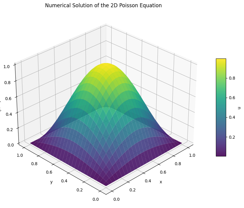
3D Surface Plot of the Numerical Solution

fig = plt.figure(figsize=(10, 7))
ax = fig.add_subplot(111, projection="3d")

surf = ax.plot_surface(X, Y, u, cmap="viridis", edgecolor="none", alpha=0.9)

ax.set_xlabel("x")
ax.set_ylabel("y")
ax.set_zlabel("u(x, y)")
ax.set_title("Numerical Solution of the 2D Poisson Equation")
fig.colorbar(surf, ax=ax, shrink=0.5, aspect=10, label="u")

ax.view_init(elev=30, azim=225)
plt.tight_layout()
plt.show()

Filled Contour Plot

fig, ax = plt.subplots(figsize=(7, 6))

levels = np.linspace(u.min(), u.max(), 30)
cf = ax.contourf(X, Y, u, levels=levels, cmap="RdYlBu_r")
ax.contour(X, Y, u, levels=10, colors="k", linewidths=0.4, alpha=0.5)

fig.colorbar(cf, ax=ax, label="u(x, y)")
ax.set_xlabel("x")
ax.set_ylabel("y")
ax.set_title("Filled Contour of the Numerical Solution")
ax.set_aspect("equal")
plt.tight_layout()
plt.show()

Comparison with the Analytical Solution

Since we chose the source term so that the exact solution is \(u(x,y) = \sin(\pi x)\sin(\pi y)\), we can compute the pointwise error and assess the accuracy of the numerical method.

error = np.abs(u - u_exact)

print(f"Maximum absolute error: {error.max():.6e}")
print(f"Mean absolute error:    {error.mean():.6e}")
print(f"RMS error:              {np.sqrt(np.mean(error**2)):.6e}")

Maximum absolute error: 2.072500e-07
Mean absolute error:    9.678488e-08
RMS error:              1.126877e-07

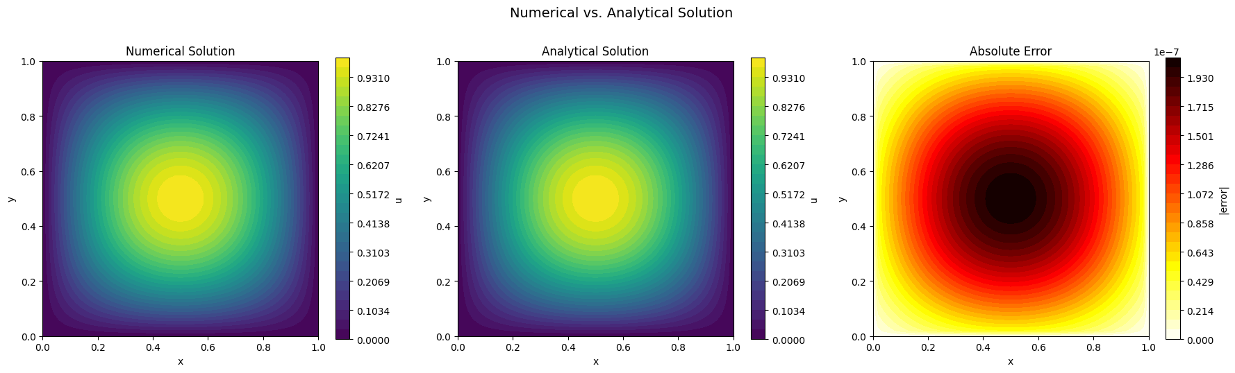
Error Distribution

fig, axes = plt.subplots(1, 3, figsize=(18, 5))

# Panel 1: Numerical solution
levels_u = np.linspace(u.min(), u.max(), 30)
cf0 = axes[0].contourf(X, Y, u, levels=levels_u, cmap="viridis")
fig.colorbar(cf0, ax=axes[0], label="u")
axes[0].set_title("Numerical Solution")
axes[0].set_xlabel("x")
axes[0].set_ylabel("y")
axes[0].set_aspect("equal")

# Panel 2: Analytical solution
cf1 = axes[1].contourf(X, Y, u_exact, levels=levels_u, cmap="viridis")
fig.colorbar(cf1, ax=axes[1], label="u")
axes[1].set_title("Analytical Solution")
axes[1].set_xlabel("x")
axes[1].set_ylabel("y")
axes[1].set_aspect("equal")

# Panel 3: Absolute error
levels_err = np.linspace(0, error.max(), 30)
cf2 = axes[2].contourf(X, Y, error, levels=levels_err, cmap="hot_r")
fig.colorbar(cf2, ax=axes[2], label="|error|")
axes[2].set_title("Absolute Error")
axes[2].set_xlabel("x")
axes[2].set_ylabel("y")
axes[2].set_aspect("equal")

plt.suptitle("Numerical vs. Analytical Solution", fontsize=14, y=1.02)
plt.tight_layout()
plt.show()

Conclusion

We have solved the 2D Poisson equation on the unit square using numgrids to construct the discrete Laplacian operator and apply Dirichlet boundary conditions. The approach is straightforward:

1. Define the grid – create coordinate axes and assemble them into a Grid object.

2. Build the operator – use Diff(grid, order, axis).as_matrix() to obtain sparse differentiation matrices and combine them into the Laplacian.

3. Apply boundary conditions – use DirichletBC and apply_bcs to modify the linear system.

4. Solve – use a standard sparse solver from SciPy.

The numerical solution closely matches the analytical result \(u(x,y) = \sin(\pi x)\sin(\pi y)\), with the error being largest near the center of the domain where the solution varies most rapidly. Increasing the number of grid points would further reduce the discretization error.