Pattern Formation: Gray-Scott and Swift-Hohenberg
Stripes, spots and labyrinths appear spontaneously in many systems: in chemical reactions, on animal coats, in convecting fluids. Two classic models of pattern formation are the Gray-Scott system of two reacting and diffusing chemicals,
and the Swift-Hohenberg equation, a model for convection rolls,
Both consist of a linear part with spatial derivatives and a local nonlinear part. On a periodic domain the linear part is diagonal in Fourier space, where it can be integrated exactly. This is what the exponential time differencing schemes of numgrids do: evolve(..., linear=L, method="ETDRK4", dt=...) steps the Fourier coefficients forward and evaluates the nonlinear terms on the grid, with fast Fourier transforms in between. The time step is then limited by the reaction terms only.
In this notebook we
grow a labyrinth from a few seeds with the Gray-Scott system and check the time step,
change two parameters and get spots that divide like cells,
let stripes and hexagons emerge from noise with the Swift-Hohenberg equation, and compare with what theory says about them.
The Gray-Scott System
The chemical \(u\) is fed at the rate \(F\) and consumed by the autocatalytic reaction \(u + 2v \to 3v\); the chemical \(v\) is removed at the rate \(F + k\). The state \(u = 1\), \(v = 0\) is stable, but a local disturbance can ignite the reaction and spread.
The linear part of a system is a nested list of operators, one row per equation. Here it contains the two diffusion terms. The right-hand side function returns the reaction terms.
[1]:
import time

import numpy as np
import matplotlib.pyplot as plt
from numgrids import *

size = 2.0
grid = Grid(x=periodic(128, 0, size), y=periodic(128, 0, size))
X, Y = grid.meshed_coords

Du, Dv = 2e-5, 1e-5
Lap = grid.laplacian_operator()
diffusion = [[Du * Lap, None],
             [None, Dv * Lap]]


def reaction(F, k):
    def rhs(t, u, v):
        uvv = u * v**2
        return -uvv + F * (1 - u), uvv - (F + k) * v
    return rhs

print(grid)
Grid(shape=(128, 128), ndims=2, axes=[
    EquidistantAxis(num_points=128, low=0, high=2.0, periodic=True, name='x'),
    EquidistantAxis(num_points=128, low=0, high=2.0, periodic=True, name='y')
])
The initial state is \(u = 1\), \(v = 0\) with a dozen seeds at random positions. The random number generator has a fixed seed, so the notebook always produces the same patterns.
[2]:
rng = np.random.default_rng(1)

seeds = np.zeros(grid.shape)
for cx, cy in rng.uniform(0.2 * size, 0.8 * size, (12, 2)):
    seeds += np.exp(-((X - cx)**2 + (Y - cy)**2) / (2 * 0.04**2))
seeds = np.minimum(seeds, 1)

u0 = 1 - 0.5 * seeds
v0 = 0.25 * seeds
A labyrinth
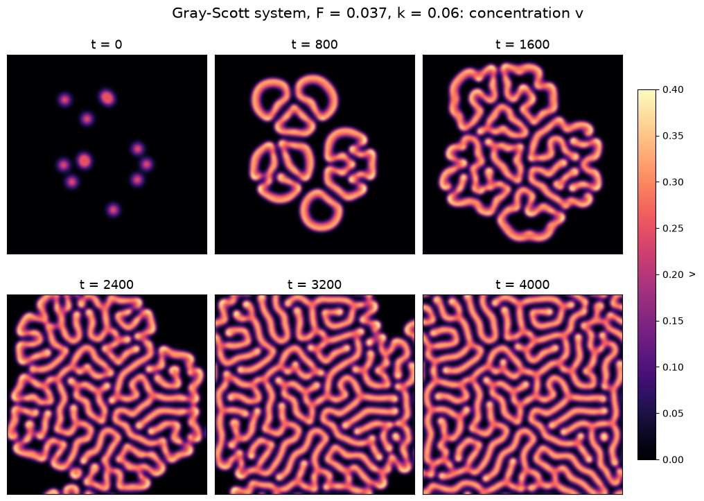
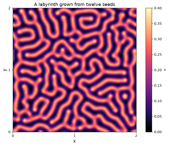
For \(F = 0.037\), \(k = 0.06\) every seed grows into a ring, the rings break up into stripes, and the stripes fill the domain with a labyrinth. We integrate up to \(t = 4000\) with the fourth-order scheme ETDRK4 and keep six snapshots.
[3]:
times = np.linspace(0, 4000, 6)

start = time.perf_counter()
labyrinth = evolve(grid, reaction(F=0.037, k=0.06), (u0, v0), t_span=(0, 4000), t_eval=times,
                   linear=diffusion, method="ETDRK4", dt=2.0)
elapsed = time.perf_counter() - start

u, v = labyrinth.u                       # each of shape (6, 128, 128)
print(labyrinth.message)
print(f"{elapsed:.1f} s for {grid.size} grid points and two fields\n")
print("     t    min(u)   max(v)   area with v > 0.15")
for t, ui, vi in zip(times, u, v):
    print(f"{t:6.0f}    {ui.min():.3f}    {vi.max():.3f}    {np.mean(vi > 0.15):6.1%}")
The integration reached the end of the time interval with 2000 steps of ETDRK4.
3.1 s for 16384 grid points and two fields

     t    min(u)   max(v)   area with v > 0.15
     0    0.500    0.250      1.7%
   800    0.264    0.388     18.3%
  1600    0.270    0.382     29.4%
  2400    0.270    0.382     44.0%
  3200    0.259    0.396     51.7%
  4000    0.264    0.379     54.6%
[4]:
def show(ax, field, title, **kwargs):
    kwargs = {"cmap": "magma", "vmin": 0, "vmax": 0.4, "interpolation": "bicubic", **kwargs}
    im = ax.imshow(field.T, origin="lower", extent=(0, size, 0, size), **kwargs)
    ax.set_title(title, fontsize=13)
    ax.set_xticks([])
    ax.set_yticks([])
    return im


fig, axes = plt.subplots(2, 3, figsize=(11, 7.5))
for ax, t, vi in zip(axes.flat, times, v):
    im = show(ax, vi, f"t = {t:.0f}")
fig.suptitle("Gray-Scott system, F = 0.037, k = 0.06: concentration v", fontsize=15)
fig.tight_layout()
fig.colorbar(im, ax=axes, shrink=0.8, pad=0.02, label="v")
plt.show()
[5]:
fig, ax = plt.subplots(figsize=(8, 6))
im = show(ax, v[-1], "A labyrinth grown from twelve seeds")
ax.set_xlabel("x", fontsize=13)
ax.set_ylabel("y", fontsize=13)
ax.set_xticks([0, 1, 2])
ax.set_yticks([0, 1, 2])
fig.colorbar(im, ax=ax, label="v")
fig.tight_layout()
plt.show()
Is the time step small enough?
The fixed-step schemes have no error control, so we check the step ourselves: repeat the first part of the run with half the step and compare. The error of a fourth-order scheme drops by a factor of 16; the difference of the two runs therefore estimates the error of the coarser one. For comparison we also run the second-order schemes ETDRK2 and IMEX2 with the same step.
[6]:
reference = evolve(grid, reaction(F=0.037, k=0.06), (u0, v0), t_span=(0, 800),
                   linear=diffusion, method="ETDRK4", dt=1.0).final[1]

print("method     dt    largest difference in v at t = 800")
print(f"ETDRK4    2.0    {np.abs(v[1] - reference).max():.1e}")
for method in ("ETDRK2", "IMEX2"):
    res = evolve(grid, reaction(F=0.037, k=0.06), (u0, v0), t_span=(0, 800),
                 linear=diffusion, method=method, dt=2.0)
    print(f"{method:6s}    2.0    {np.abs(res.final[1] - reference).max():.1e}")
method     dt    largest difference in v at t = 800
ETDRK4    2.0    1.6e-05
ETDRK2    2.0    1.0e-02
IMEX2     2.0    3.8e-03
With \(\Delta t = 2\) the snapshots of ETDRK4 are accurate to about five digits. A step of this size is possible because diffusion is integrated exactly; the reaction terms change on a time scale of \(1/(F + k) \approx 10\).
Dividing spots
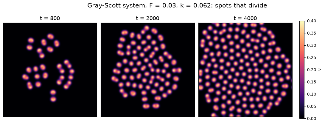
A small change of the parameters gives a different pattern. For \(F = 0.03\), \(k = 0.062\) the stripes are unstable: every seed turns into spots, and the spots divide like cells until they fill the domain.
[7]:
start = time.perf_counter()
spots = evolve(grid, reaction(F=0.03, k=0.062), (u0, v0), t_span=(0, 4000), t_eval=[800, 2000, 4000],
               linear=diffusion, method="ETDRK4", dt=2.0)
print(f"{spots.message}  ({time.perf_counter() - start:.1f} s)")

fig, axes = plt.subplots(1, 3, figsize=(12, 4.3))
for ax, t, vi in zip(axes, spots.t, spots.u[1]):
    im = show(ax, vi, f"t = {t:.0f}")
fig.suptitle("Gray-Scott system, F = 0.03, k = 0.062: spots that divide", fontsize=15)
fig.tight_layout()
fig.colorbar(im, ax=axes, shrink=0.9, pad=0.02, label="v")
plt.show()
The integration reached the end of the time interval with 2000 steps of ETDRK4. (3.1 s)
The Swift-Hohenberg Equation
The linear part \(r - (1 + \nabla^2)^2\) of the Swift-Hohenberg equation amplifies Fourier modes \(e^{i \mathbf{k} \cdot \mathbf{x}}\) with the rate
so for \(r > 0\) a band of modes around \(|\mathbf{k}| = 1\) grows, and the nonlinear terms decide which pattern they form.
The operator contains the mixed derivative \(\partial_x^2 \partial_y^2\). Its matrix is dense: it would have \(128^4 \approx 2.7 \cdot 10^8\) entries here. On periodic grids there is a way around the matrix: the linear part can be given as its Fourier symbol, the function \(\sigma\) of the wave numbers.
The fourth derivative makes this problem stiff. The fastest decaying mode has the rate \(-960\), which limits explicit methods to steps of about \(0.003\). We use \(\Delta t = 0.5\).
[8]:
size = 32 * np.pi                        # 16 wavelengths of the critical mode
grid = Grid(x=periodic(128, 0, size), y=periodic(128, 0, size))

rng = np.random.default_rng(2)
noise = 0.01 * rng.standard_normal(grid.shape)


def swift_hohenberg(r, g, t_end, t_eval=None):
    return evolve(grid, lambda t, u: g * u**2 - u * u**2, noise, t_span=(0, t_end), t_eval=t_eval,
                  linear=lambda kx, ky: r - (1 - kx**2 - ky**2)**2, method="ETDRK4", dt=0.5)


start = time.perf_counter()
stripes = swift_hohenberg(r=0.3, g=0.0, t_end=300, t_eval=[0, 5, 300])
hexagons = swift_hohenberg(r=0.1, g=1.0, t_end=500)
print(stripes.message)
print(hexagons.message)
print(f"{time.perf_counter() - start:.1f} s")
The integration reached the end of the time interval with 600 steps of ETDRK4.
The integration reached the end of the time interval with 1000 steps of ETDRK4.
1.3 s
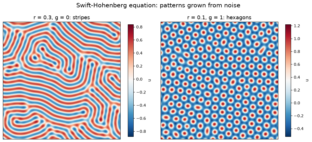
Without the quadratic term (\(g = 0\)) the equation is symmetric under \(u \to -u\) and forms stripes. The quadratic term breaks this symmetry and favors hexagons.
[9]:
fig, axes = plt.subplots(1, 2, figsize=(11, 5.2))
for ax, res, title in [(axes[0], stripes, "r = 0.3, g = 0: stripes"),
                       (axes[1], hexagons, "r = 0.1, g = 1: hexagons")]:
    im = show(ax, res.final, title, cmap="RdBu_r", vmin=None, vmax=None)
    fig.colorbar(im, ax=ax, shrink=0.85, label="u")
fig.suptitle("Swift-Hohenberg equation: patterns grown from noise", fontsize=15)
fig.tight_layout()
plt.show()
Comparison with theory
Two exact statements can be checked.
Linear growth. As long as \(u\) is small, the nonlinear terms are negligible, and every Fourier mode of the noise grows exactly with its rate \(\sigma(\mathbf{k})\). The scheme integrates the linear part without error, so the numerical solution must follow this law. We compare the Fourier coefficients at \(t = 5\) with the prediction.
Wave number. The fastest growing modes have \(|\mathbf{k}| = 1\), so the stripes should have the wave length \(2\pi\).
[10]:
k = 2 * np.pi * np.fft.fftfreq(128, d=size / 128)
KX, KY = np.meshgrid(k, k, indexing="ij")
sigma = 0.3 - (1 - KX**2 - KY**2)**2

predicted = np.exp(5 * sigma) * np.fft.fft2(noise)
computed = np.fft.fft2(stripes.u[1])
print(f"growth of the noise up to t = 5: largest deviation from exp(sigma t) = "
      f"{np.abs(computed - predicted).max() / np.abs(predicted).max():.1e}")

power = np.abs(np.fft.fft2(stripes.final))**2
print(f"mean wave number of the stripes: {np.sum(np.hypot(KX, KY) * power) / np.sum(power):.3f}")
growth of the noise up to t = 5: largest deviation from exp(sigma t) = 3.5e-04
mean wave number of the stripes: 0.993
The first number is not zero because the cubic term already acts on the growing noise: it is of the order \(u^2 \approx 10^{-4}\).
Energy. The Swift-Hohenberg equation is a gradient flow: it only ever decreases the functional
grid.laplacian and grid.integrate evaluate it for the snapshots of a run:
[11]:
def energy(u, r, g):
    return grid.integrate(0.5 * (u + grid.laplacian(u))**2 - r / 2 * u**2 - g / 3 * u**3 + u**4 / 4)


times = [0, 20, 40, 60, 100, 200, 500]
run = swift_hohenberg(r=0.1, g=1.0, t_end=500, t_eval=times)
values = [energy(u, 0.1, 1.0) for u in run.u]

print("    t      energy")
for t, value in zip(times, values):
    print(f"{t:5.0f}   {value:10.4f}")
print("decreasing:", bool(np.all(np.diff(values) < 0)))
    t      energy
    0      71.5914
   20      -0.0309
   40      -1.9578
   60    -113.6092
  100    -132.1342
  200    -136.6064
  500    -138.9254
decreasing: True
Summary
evolve(grid, N, u0, t_span, linear=L, method="ETDRK4", dt=...)integrates stiff semilinear problems with a fixed step: the linear part exactly, the nonlinear part with a fourth-order Runge-Kutta scheme.For systems,
linearis a nested list of operators and the nonlinear part returns one array per field.On periodic grids, linear parts with constant coefficients are handled in Fourier space. Two fields on a \(128 \times 128\) grid take a few milliseconds per step.
Operators with dense matrices, like \((1 + \nabla^2)^2\) in two dimensions, can be passed as Fourier symbols:
linear=lambda kx, ky: r - (1 - kx**2 - ky**2)**2.There is no error control. Check the time step by comparing with a run with half the step.