Nonlinear Boundary Value Problems
Many steady-state problems are nonlinear: reaction terms such as \(e^u\), conductivities that depend on the temperature, equilibria of reaction-diffusion systems. In this notebook we solve such problems with solve_nonlinear, which applies Newton’s method to a residual \(F(u) = 0\) that we write down with the usual numgrids tools.
We will
solve the Bratu problem and compare with its exact solution,
find both of its solutions, follow the whole solution branch through its fold with continuation, and see which of the solutions are stable,
speed things up with an exact Jacobian written in operator algebra,
solve the Bratu problem on the full unit disk, and
compute the temperature in a plate with a temperature-dependent conductivity.
[1]:
import time

import matplotlib.pyplot as plt
import numpy as np
from scipy.optimize import brentq

from numgrids import *
from numgrids.nonlinear import continuation, linear_stability
1. The Bratu Problem
The Bratu problem
is a classic model of thermal runaway in a reactive slab: the reaction heats the material, and the reaction rate grows exponentially with the temperature. For \(\lambda = 1\) we pass the residual \(F(u) = u'' + \lambda e^u\), an initial guess and the boundary conditions. With verbose=True we watch Newton’s method converge quadratically.
[2]:
grid = Grid(x=chebyshev(41, 0, 1))
x = grid.coords

u = solve_nonlinear(grid, lambda u: grid.diff(u, 2) + np.exp(u), u0=0, bcs=0, verbose=True)
Newton step 1: |F| = 1.020e-02, |du| = 1.395e-01, damping = 1
Newton step 2: |F| = 6.166e-07, |du| = 1.045e-03, damping = 1
Newton step 3: |F| = 1.434e-11, |du| = 5.879e-08, damping = 1
Newton step 4: |F| = 6.930e-13, |du| = 6.182e-14, damping = 1
The exact solution is \(u(x) = -2 \ln\left(\cosh\bigl((x - \tfrac12)\tfrac{\theta}{2}\bigr) / \cosh\tfrac{\theta}{4}\right)\), where \(\theta\) solves \(\theta = \sqrt{2\lambda}\,\cosh(\theta/4)\). That equation has two roots, which belong to two different solutions. We come back to that below.
[3]:
def bratu_exact(x, lam, branch="lower"):
    f = lambda t: t - np.sqrt(2 * lam) * np.cosh(t / 4)
    theta = brentq(f, 0, 5) if branch == "lower" else brentq(f, 5, 30)
    return -2 * np.log(np.cosh((x - 0.5) * theta / 2) / np.cosh(theta / 4))

print("max. error:", np.max(np.abs(u - bratu_exact(x, 1.0))))
max. error: 3.635980405647388e-15
2. Two Solutions and Continuation
Newton’s method converges to a solution near the initial guess. Starting from a large bump, we find the second solution of the Bratu problem for the same \(\lambda = 1\):
[4]:
upper = solve_nonlinear(grid, lambda u: grid.diff(u, 2) + np.exp(u),
                        u0=4 * np.sin(np.pi * x), bcs=0)
print("max. error:", np.max(np.abs(upper - bratu_exact(x, 1.0, "upper"))))

fig, ax = plt.subplots(figsize=(8, 4.5))
xf = np.linspace(0, 1, 300)
for sol, name, color in [(u, "lower", "tab:blue"), (upper, "upper", "tab:red")]:
    ax.plot(xf, bratu_exact(xf, 1.0, name), color=color, lw=2, label=f"exact ({name} branch)")
    ax.plot(x, sol, "o", color=color, ms=4, label=f"numgrids ({name} branch)")
ax.set_xlabel("$x$")
ax.set_ylabel("$u(x)$")
ax.set_title(r"The two solutions of $u'' + e^u = 0$")
ax.legend()
plt.show()
max. error: 1.0816236795108125e-11
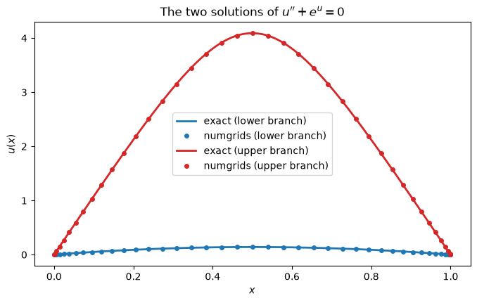
How are the two solutions related, and what happens for other values of \(\lambda\)? continuation follows a branch of solutions of \(F(u, \lambda) = 0\), starting from the solution for one value of the parameter. The residual takes the parameter as its last argument. We start from the trivial solution \(u = 0\) at \(\lambda = 0\) and take 150 steps of length ds = 0.05 along the branch.
With stability=3, the continuation also computes the three leading eigenvalues of the Jacobian at every point. They tell whether the solution is stable as a steady state of the reaction-diffusion equation \(u_t = u'' + \lambda e^u\): a small perturbation grows like \(e^{\sigma t}\) with the eigenvalues \(\sigma\), so the solution is stable if all eigenvalues are negative.
[5]:
def bratu(u, lam):
    return grid.diff(u, 2) + lam * np.exp(u)

branch = continuation(grid, bratu, u0=0, param=0, bcs=0, ds=0.05, max_steps=150, stability=3)
max_u = branch.measure(np.max)

print(branch)
print("solutions:", branch.u.shape, "(point on the branch, x)")
print("lambda:   ", np.round(branch.params[:3], 4), "...", np.round(branch.params[71:76], 4),
      "...", np.round(branch.params[-3:], 4))
print("max u:    ", np.round(max_u[:3], 4), "...", np.round(max_u[71:76], 4),
      "...", np.round(max_u[-3:], 4))
print("stable:   ", branch.stable[:3], "...", branch.stable[71:76], "...", branch.stable[-3:])
print("folds:    ", branch.folds)
ContinuationResult(151 points, parameter from 0 to 0.440556, 1 fold(s), 74 stable point(s), success=True)
solutions: (151, 41) (point on the branch, x)
lambda:    [0.     0.0499 0.0997] ... [3.4707 3.4995 3.5134 3.5077 3.4868] ... [0.4947 0.4672 0.4406]
max u:     [0.     0.0063 0.0126] ... [1.0111 1.0833 1.169  1.258  1.3392] ... [5.1511 5.2336 5.3175]
stable:    [ True  True  True] ... [ True  True  True False False] ... [False False False]
folds:     [73]
branch.params holds the parameters and branch.u the solutions along the branch, and branch.measure(func) reduces every solution to a number, here its maximum. The parameter increases up to \(\lambda \approx 3.51\) and then decreases again, while the solutions keep growing: the branch turns back in a fold. branch.folds lists the points of the branch where this happens. Up to the fold the solutions are stable, behind it they are not.
The fold itself lies between two points of the branch. continuation locates it there, by solving for the point of the branch where the parameter is stationary: branch.fold_params and branch.fold_u hold the parameters and the solutions at the folds. We compare with the exact curve, which is known in terms of the parameter \(\theta\) of the exact solution, \(\lambda = \theta^2 / \bigl(2 \cosh^2 (\theta/4)\bigr)\) and \(\max u = 2 \ln \cosh (\theta/4)\). Its fold is at
\(\lambda_c = 3.513830719\ldots\)
[6]:
k = branch.folds[0]
lam_fold = branch.fold_params[0]
max_u_fold = branch.fold_u[0].max()
print(f"point {k} of the branch:  lambda = {branch.params[k]:.10f},  max u = {max_u[k]:.8f}")
print(f"located fold:            lambda = {lam_fold:.10f},  max u = {max_u_fold:.8f}")

# The exact fold: the maximum of lambda(theta) is at theta = 4 s with s tanh(s) = 1
s = brentq(lambda s: s * np.tanh(s) - 1, 1, 2)
lam_c = 8 * s**2 / np.cosh(s) ** 2
print(f"exact:                   lambda = {lam_c:.10f},  max u = {2 * np.log(np.cosh(s)):.8f}")

# All points of the branch must lie on the exact curve lambda(max u)
theta = 4 * np.arccosh(np.exp(max_u / 2))
print("largest deviation of the branch from the exact curve:",
      f"{np.max(np.abs(branch.params - theta**2 / (2 * np.cosh(theta / 4) ** 2))):.1e}")
point 73 of the branch:  lambda = 3.5134239741,  max u = 1.16899409
located fold:            lambda = 3.5138307191,  max u = 1.18684217
exact:                   lambda = 3.5138307191,  max u = 1.18684217
largest deviation of the branch from the exact curve: 2.2e-10
The bifurcation diagram shows \(\max u\) against \(\lambda\), as usual with a solid line for the stable and a dashed line for the unstable solutions. The two solutions for \(\lambda = 1\) from above are the lower and the upper part of one and the same branch, and beyond the fold there is no solution at all.
[7]:
theta = np.linspace(0.01, 16, 500)
lam_exact = theta**2 / (2 * np.cosh(theta / 4) ** 2)
max_exact = 2 * np.log(np.cosh(theta / 4))

# The stable and the unstable part of the branch meet in the fold
stable, unstable = branch.stable, ~branch.stable
lam_stable = np.append(branch.params[stable], lam_fold)
lam_unstable = np.append(lam_fold, branch.params[unstable])

fig, ax = plt.subplots(figsize=(8, 5))
ax.plot(lam_exact, max_exact, "-", color="0.8", lw=7, label="exact")
ax.plot(lam_stable, np.append(max_u[stable], max_u_fold), "-", color="tab:green", lw=2,
        label="continuation, stable")
ax.plot(lam_unstable, np.append(max_u_fold, max_u[unstable]), "--", color="tab:green", lw=2,
        label="continuation, unstable")
ax.plot(1.0, u.max(), "o", color="tab:blue", ms=9, label=r"lower solution for $\lambda = 1$")
ax.plot(1.0, upper.max(), "s", color="tab:red", ms=8, label=r"upper solution for $\lambda = 1$")
ax.plot(lam_fold, max_u_fold, "*", color="gold", mec="k", ms=18,
        label=rf"fold, $\lambda_c = {lam_fold:.4f}$")
ax.axvline(lam_fold, color="gray", ls=":", lw=1)
ax.set_xlabel(r"$\lambda$")
ax.set_ylabel(r"$\max\, u$")
ax.set_title("Bifurcation diagram of the Bratu problem")
ax.legend(loc="upper right", bbox_to_anchor=(0.93, 1.0))
plt.show()
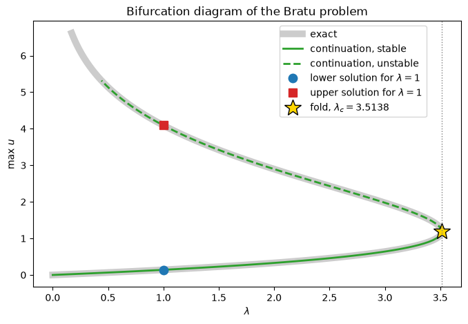
The stability changes exactly at the fold: there the leading eigenvalue branch.eigenvalues[:, 0] crosses zero. Behind the fold one perturbation grows, and the temperature either runs away or falls back to the lower solution. For a single solution, linear_stability gives the same information.
[8]:
fig, ax = plt.subplots(figsize=(8, 4))
ax.axhline(0, color="gray", lw=1)
ax.plot(max_u, branch.eigenvalues[:, 0], "o-", color="tab:green", ms=3, label="points of the branch")
ax.plot(max_u_fold, 0, "*", color="gold", mec="k", ms=18, label="fold")
ax.set_xlabel(r"$\max\, u$ (increases along the branch)")
ax.set_ylabel(r"leading eigenvalue $\sigma_1$")
ax.legend()
plt.show()

print(branch.bifurcations)
for name, solution in [("lower", u), ("upper", upper)]:
    print(f"{name} solution for lambda = 1:", linear_stability(grid, bratu, solution, bcs=0, param=1.0))
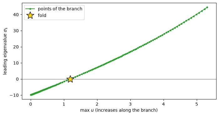
[Bifurcation(fold at param = 3.513830719, between the points 73 and 74)]
lower solution for lambda = 1: StabilityResult(stable, growth rate -8.7397)
upper solution for lambda = 1: StabilityResult(unstable, 1 unstable mode, growth rate 28.873)
Could we have traced this diagram with solve_nonlinear alone, increasing \(\lambda\) step by step and using each solution as the initial guess for the next? Only in pieces. Stepping in the parameter cannot pass a fold: the Jacobian is singular there, and behind it the parameter has to decrease again. One would have to stop short of the fold and start the upper branch from a separately found solution. continuation steps along the curve \((u, \lambda)\) itself (pseudo-arclength
continuation) and treats the parameter as an unknown like the solution, so it passes the fold in one go.
Beyond the fold, for \(\lambda > \lambda_c\), Newton’s method cannot converge. solve_nonlinear then raises a NonlinearSolverError, which carries the last iterate and the residual history:
[9]:
try:
    solve_nonlinear(grid, lambda u: bratu(u, 4.0), 0, bcs=0, maxiter=20)
except NonlinearSolverError as err:
    print(err)
    print("last residuals:", np.round(err.residuals[-3:], 3))
Newton's method did not converge in 20 steps (residual 1.935e+00). Try a better initial guess (e.g. continuation from a nearby problem).
last residuals: [1.933 1.933 1.935]
3. An Exact Jacobian
Newton’s method needs the Jacobian \(J = \partial F / \partial u\). By default, solve_nonlinear approximates it by finite differences, which costs one residual evaluation per grid point and Newton step. For larger grids we pass the exact Jacobian instead. Thanks to the operator algebra it looks just like the formula: for \(F(u) = \nabla^2 u + \lambda e^u\), the Jacobian is \(J = \nabla^2 + \lambda e^u\) (an operator plus a multiplication). Here is the Bratu problem on a square:
[10]:
square = Grid(x=chebyshev(40, 0, 1), y=chebyshev(40, 0, 1))
L = square.laplacian_operator()
lam = 6.0

start = time.perf_counter()
u_fd = solve_nonlinear(square, lambda u: L(u) + lam * np.exp(u), 0, bcs=0)
t_fd = time.perf_counter() - start

start = time.perf_counter()
u_ex = solve_nonlinear(square, lambda u: L(u) + lam * np.exp(u), 0, bcs=0,
                       jacobian=lambda u: L + lam * np.exp(u))
t_ex = time.perf_counter() - start

print(f"finite-difference Jacobian: {t_fd:.3f} s")
print(f"exact Jacobian:             {t_ex:.3f} s")
print("difference of the solutions:", np.max(np.abs(u_fd - u_ex)))
finite-difference Jacobian: 1.571 s
exact Jacobian:             0.429 s
difference of the solutions: 1.7763568394002505e-15
4. The Bratu Problem on the Full Disk
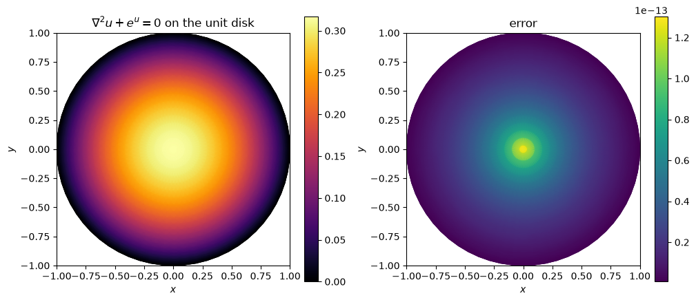
Everything works on curvilinear grids, too. On the unit disk, the Bratu problem \(\nabla^2 u + \lambda e^u = 0\) with \(u = 0\) on the rim has the exact solution
A PolarGrid with a radial axis covers the full disk including its center. The only boundary is the rim.
[11]:
disk = PolarGrid(radial(24, 1.0), periodic(64))
L = disk.laplacian_operator()
lam = 1.0

u = solve_nonlinear(disk, lambda u: L(u) + lam * np.exp(u), 0, bcs=0,
                    jacobian=lambda u: L + lam * np.exp(u))

R, _ = disk.meshed_coords
mu = (4 / lam - 1) - np.sqrt((4 / lam - 1) ** 2 - 1)        # the smaller root
exact = np.log(8 * mu / lam / (1 + mu * R**2) ** 2)
print("max. error:", np.max(np.abs(u - exact)))

fig, axes = plt.subplots(1, 2, figsize=(12, 5))
disk.plot(u, ax=axes[0], cmap="inferno")
axes[0].set_title(r"$\nabla^2 u + e^u = 0$ on the unit disk")
disk.plot(np.abs(u - exact), ax=axes[1], cmap="viridis")
axes[1].set_title("error")
plt.show()
max. error: 1.249000902703301e-13
5. A Plate with Temperature-Dependent Conductivity
In many materials the thermal conductivity depends on the temperature. The steady temperature in a plate heated uniformly with power density \(q\) then satisfies
We take \(k(u) = 1 + u^2\) (a conductivity that grows with the temperature) and keep three edges at temperature 0. The top edge is insulated, \(\partial u / \partial n = 0\). The residual is a direct transcription of the equation.
[12]:
plate = Grid(x=chebyshev(24, 0, 2), y=chebyshev(24, 0, 1))
q = 20.0

def k(u):
    return 1 + u**2

def residual(u):
    flux = [k(u) * g for g in plate.gradient(u)]
    return plate.divergence(*flux) + q

bcs = {"x_low": 0, "x_high": 0, "y_low": 0, "y_high": Neumann(0)}
u = solve_nonlinear(plate, residual, 0, bcs=bcs)

# For comparison: constant conductivity k = 1 (a linear problem)
u_lin = plate.laplacian_operator().solve(-q, bcs=bcs)

fig, axes = plt.subplots(2, 1, figsize=(8, 8), constrained_layout=True)
for ax, f, title in [(axes[0], u_lin, "constant conductivity $k = 1$"),
                     (axes[1], u, "$k(u) = 1 + u^2$")]:
    plate.plot(f, ax=ax, cmap="inferno")
    ax.set_title(f"{title}: max $u$ = {f.max():.3f}")
    ax.set_aspect("equal")
plt.show()

# Temperature along the vertical center line x = 1
y_line = np.linspace(0, 1, 100)
points = np.column_stack([np.ones_like(y_line), y_line])
fig, ax = plt.subplots(figsize=(8, 4))
ax.plot(y_line, plate.interpolate(u_lin, points, method="spectral"), lw=2, label="$k = 1$")
ax.plot(y_line, plate.interpolate(u, points, method="spectral"), lw=2, label="$k(u) = 1 + u^2$")
ax.set_xlabel("$y$ (insulated edge at $y = 1$)")
ax.set_ylabel("$u(1, y)$")
ax.legend()
plt.show()
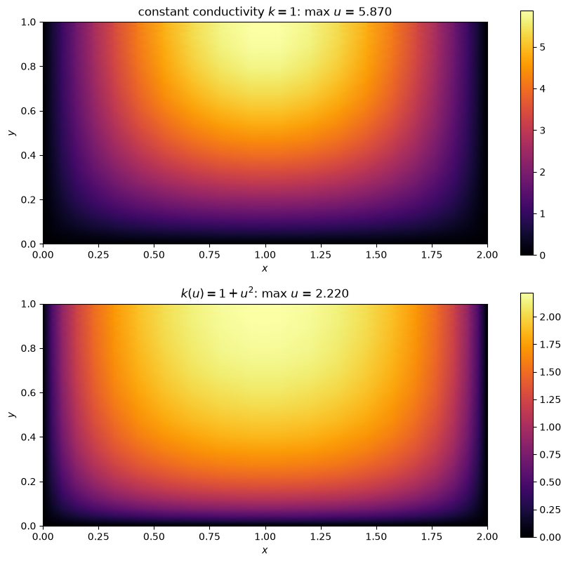
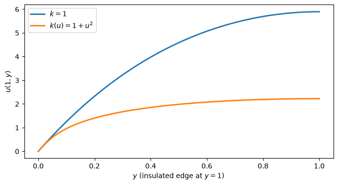
The hotter the material, the better it conducts. So the plate with temperature-dependent conductivity stays cooler than the one with constant conductivity, and its temperature profile is flatter. On both plates the temperature is highest at the insulated top edge, where its normal derivative vanishes: no heat can escape there.
Summary
solve_nonlinear solves nonlinear boundary value problems with Newton’s method:
u = solve_nonlinear(grid, residual, u0, bcs=..., jacobian=...)
The residual is an ordinary function of grid-shaped arrays, written with
grid.diff,grid.gradient, operators and NumPy functions.The initial guess selects the solution when there are several of them.
continuationfollows a branch of solutions while a parameter changes, through folds, and finds how the solutions are connected. It locates the folds and, withstability=k, tells which solutions are stable;linear_stabilitydoes so for a single solution.Boundary conditions take the same compact forms as for
solveandevolve(Dirichlet, Neumann, Robin).Without further information the Jacobian is computed by finite differences. An exact Jacobian is quickly written with operator algebra and is much faster for larger grids.
Everything works on curvilinear grids, including the full disk.
Coupled systems of equations are supported as well, see the user guide.