Theory

As the name findiff suggests, the package uses finite difference schemes to approximate differential operators numerically.

Notation

Consider functions defined on equidistant grids.

In 1D, instead of a continuous variable \(x\), we have a set of grid points

\[x_i = a + i \Delta x\]

for some real number \(a\) and grid spacing \(\Delta x\). In many dimensions, say 3, we have

\[\begin{split}x_{ijk} = \left( \begin{matrix} x_i \\ y_j \\ z_k \\ \end{matrix} \right) = \left( \begin{matrix} a_x + i \Delta x \\ a_y + j \Delta y \\ a_z + k \Delta z \\ \end{matrix} \right)\end{split}\]

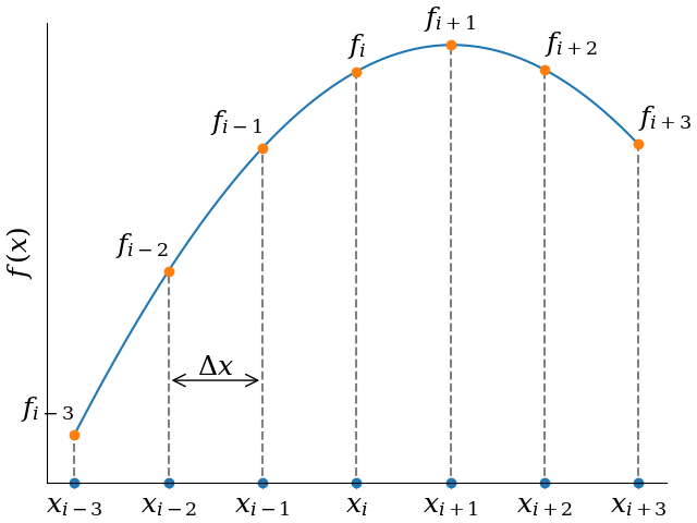
For a function f given on a grid, we write

\[f_{ijk} = f(x_{ijk})\]

The generalization to N dimensions is straightforward.

The 1D Case

Say we want to calculate the n-th derivative \(\frac{d^n f}{dx^n}\) of a function of a single variable given on an equidistant grid. The basic idea behind finite differences is to approximate the derivative at some point \(x_k\) by a linear combination of function values around \(x_k\):

\[\left(\frac{d^n f}{dx^n}\right)_k = f^{(n)}_k \approx \sum_{j \in A} c_{j} f_{k+j}\]

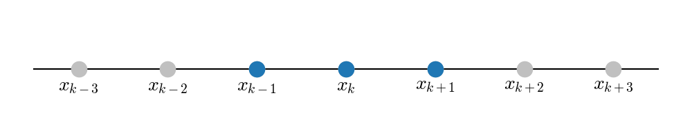
where A is a set of offsets, such that \(k+j\) are indices of grid points neighboring \(x_k\). Specifically, let \(A=\{-p, -p+1, \ldots, q-1, q\}\) for positive integers \(p, q \ge 0\). For \(p=q=1\), we use the following grid points:

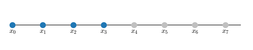
This is a symmetric stencil. It does not work if \(x_k\) is at the boundary of the grid, because there would be no points to one side. In that case, we use a one-sided stencil like this forward stencil (\(p=0, q=3\)):

For \(f_{k+j}\) we insert the Taylor expansion around \(f_k\):

\[f_{k+j} = \sum_{\alpha=0}^\infty \frac{1}{\alpha !} (j \Delta x)^\alpha f^{(\alpha)}_k\]

So we have

\[f^{(n)}_k \approx \sum_{\alpha=0}^\infty \underbrace{\left(\sum_{j=-p}^q c_{j} j^\alpha \right) \frac{\Delta x^\alpha}{\alpha !}}_{M_\alpha} f^{(\alpha)}_k\]

Demanding \(M_\alpha = \delta_{n\alpha}\) yields the system of equations:

\[\sum_{j=-p}^q c_{j} j^\alpha = \frac{\alpha !}{\Delta x^\alpha} \delta_{n\alpha}\]

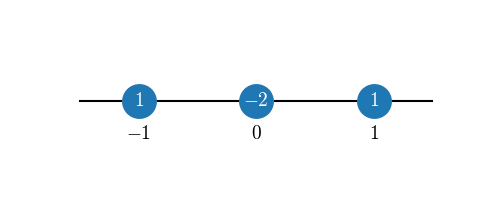
For example, a symmetric scheme with \(p=q=1\) for the second derivative gives:

\[\begin{split}\left( \begin{matrix} 1 & 1 & 1 \\ -1 & 0 & 1 \\ 1 & 0 & 1 \end{matrix} \right) \left( \begin{matrix} c_{-1} \\ c_0 \\ c_1 \end{matrix} \right) = \left( \begin{matrix} 0 \\ 0 \\ 2 \end{matrix} \right)\end{split}\]

with solution \(c_{-1} = c_1 = 1, \quad c_0 = -2\):

\[\left(\frac{d^2 f}{dx^2}\right)_k \approx \frac{f_{k-1} - 2f_k + f_{k+1}}{\Delta x^2}\]

This has second order accuracy, i.e. the error is \(\mathcal{O}(\Delta x^2)\).

Compact stencil visualization:

Multiple Dimensions

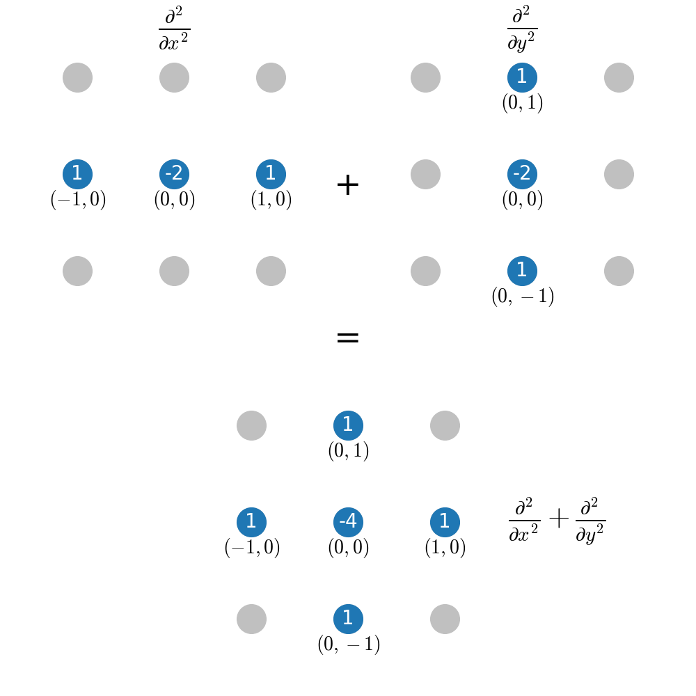
For functions of several variables, the same idea applies to partial derivatives using linear combinations of neighboring grid points. In most cases the optimal stencil is a superposition of 1D stencils. For example, the 2D Laplacian:

\[\frac{\partial^2}{\partial x^2} + \frac{\partial^2}{\partial y^2}\]

uses a cross-shaped stencil composed of two 1D stencils:

Non-Uniform Grids

On a non-uniform grid the spacing varies: \(\Delta x_i = x_{i+1} - x_i\) is not constant. The Taylor expansion approach still works, but the offsets \(j \Delta x\) are replaced by the actual distances \(x_{k+j} - x_k\):

\[f_{k+j} = \sum_{\alpha=0}^{\infty} \frac{(x_{k+j} - x_k)^\alpha}{\alpha!}\, f^{(\alpha)}_k\]

The coefficient system becomes:

\[\sum_{j} c_j\, (x_{k+j} - x_k)^\alpha = \delta_{n\alpha}\, \alpha!\]

Because the distances differ at every grid point, the coefficients \(c_j\) depend on the location \(k\). findiff solves this system at each point automatically when a coordinate array (instead of a scalar spacing) is passed to Diff.

Compact (Implicit) Finite Differences

Standard (“explicit”) finite differences express the derivative as a weighted sum of function values alone:

\[f'_i = \sum_k c_k \, f_{i+k}\]

To reach high accuracy the stencil must be wide (many points), which increases both computational cost and sensitivity to noise.

Compact finite differences generalize this by including derivative values on the left-hand side:

\[\sum_k \alpha_k \, f'_{i+k} = \sum_k c_k \, f_{i+k}\]

The classic tridiagonal scheme (Lele, 1992) sets \(\alpha_{-1} = \alpha_1 = \tfrac{1}{3}\) and uses a seven-point right-hand side. Despite involving only nearest-neighbor derivative coupling, it achieves 6th-order accuracy — the same as a 7-point explicit stencil.

How the coefficients are determined. Given the left-hand side coefficients \(\alpha_k\) and a set of right-hand side offsets, insert Taylor expansions for both \(f'_{i+k}\) and \(f_{i+k}\) around \(x_i\) and match powers of \(\Delta x\) up to the desired order. This yields a linear system for the \(c_k\), analogous to the explicit case but with additional constraints from the left-hand side.

Trade-off. Applying a compact operator requires solving a banded linear system (e.g. tridiagonal). For a tridiagonal left-hand side this costs \(O(N)\) via the Thomas algorithm, so the overhead is modest. In return the scheme resolves short-wavelength features much more accurately than an explicit scheme with the same stencil width.

See the Compact Finite Differences guide for usage details and the reference:

S. K. Lele, “Compact Finite Difference Schemes with Spectral-like Resolution”, J. Comp. Phys. 103, 16–42 (1992).

Error Estimation

A finite difference approximation of accuracy order \(p\) satisfies

\[f'_{\mathrm{FD}} = f'_{\mathrm{exact}} + C\,h^p + \mathcal{O}(h^{p+2})\]

where \(C\) depends on higher derivatives of \(f\) and on the scheme, and \(h = \Delta x\). The leading error term \(C\,h^p\) is not directly accessible because \(f'_{\mathrm{exact}}\) is unknown.

However, computing the same derivative at two consecutive accuracy orders \(p\) and \(p+2\) gives:

\[\begin{split}f'_{(p)} &= f'_{\mathrm{exact}} + C\,h^p + \mathcal{O}(h^{p+2}) \\ f'_{(p+2)} &= f'_{\mathrm{exact}} + C'\,h^{p+2} + \mathcal{O}(h^{p+4})\end{split}\]

Subtracting:

\[\left| f'_{(p)} - f'_{(p+2)} \right| \approx |C|\,h^p\]

This difference is a pointwise estimate of the truncation error at order \(p\). The higher-order result \(f'_{(p+2)}\) is itself a better approximation and is returned as the extrapolated value.

This technique is a simplified form of Richardson extrapolation. It does not require evaluating on a second, finer grid — instead it widens the stencil to gain two extra orders of accuracy and uses the difference as the error indicator.

See the Error Estimation guide for the API.